Overview
This tutorial is about modeling two-way flow, also called bidirectional flow. Two-way flow is relevant to certain transient contamination studies performed with Ventus, ContamW, and other tools.
This topic is relevant to you if you are modeling contaminant transport through tall openings that connect different temperature rooms.
In this example, mathematical models are presented and discussed.
Before Starting
- Review the Modeling Contaminants tutorial.
- Download the
two-way flow zipto follow along. The ZIP folder includes:2-zone-contaminant.vntsand in Solutiontwo-way-flow-finished.vnts
Introduction
Create a simple two-Zone model to calculate two-way flow and understand the significance of the Flow Element models. Work through an example, drawing from the guidance found in the ASHRAE Handbook of Smoke Control, the REHVA Smoke Management Guidelines, and CONTAM documentation.
- First, create a One-way Flow Simulation.
- Second, create a Two-way Flow Simulation.
- Third, Introduce External Pressure .
Theory
A compartment fire drives air flow around it through buoyancy and pressure differentials. Any Zone that contains the fire and smoke path will have an extreme three-dimensional temperature gradient.
This gradient will drive flow across any large vertical openings between the fire compartment and an outside compartment. Flow characteristics will depend on the neutral plane height for both compartment one and compartment two.
Temperature differences and connections through tall vertical openings between zones can cause horizontal flow between those zones. Air, like water, is a fluid that is self-levelling; warm air will spill through openings and fill ceilings like an upside down bathtub; cold air will spill through openings in the opposite direction. At a building scale, this results in stack effect.
According to the CONTAM documentation, a doorway, or even a window, may be better characterized by a two-way flow model. Temperature differences between Zones drive vertical density gradients that create small horizontal pressure differentials across the height of openings. (Dols and Polidoro 2020)
Flow characteristics will depend on the neutral plane height; two-way flow is only possible when the neutral plane of flow is within the height of the opening. To consider these conditions and assess flow characteristics, isolate the flow as done in the CONTAM Technical Reference. The hydrostatic equation is used to calculate pressure differentials resulting from the temperature difference. (Walton 1989).
For the idealized case, in a lumped-parameter model, when no external pressures are applied:
 |  |
From Figure 2, Figure 3, and Figure 4:
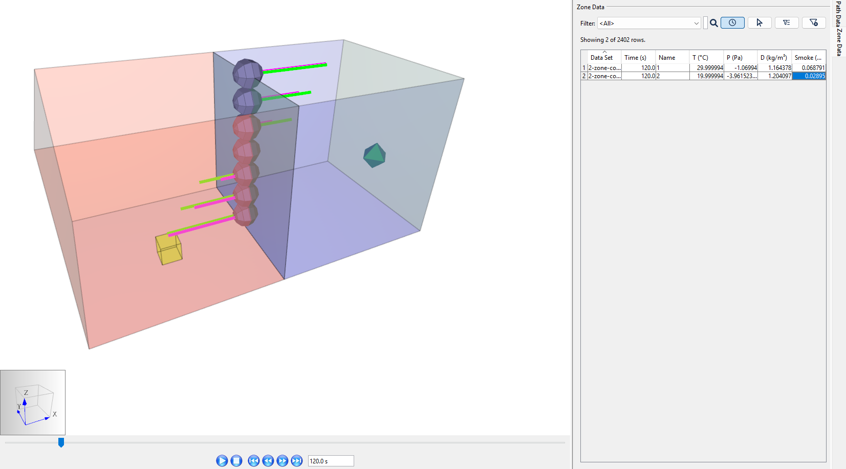
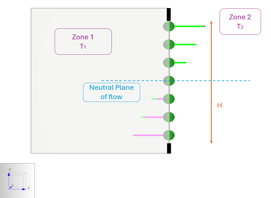
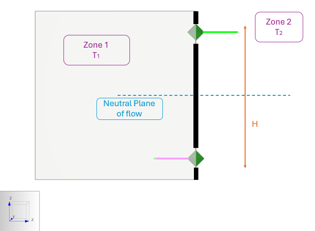
- Bidirectional flow can be modeled with a continuous opening or with two opposite-direction openings.
- In cases where the Zones are aligned horizontally, such that hneutral_plane = hmid_opening, the net mass flow is 0.
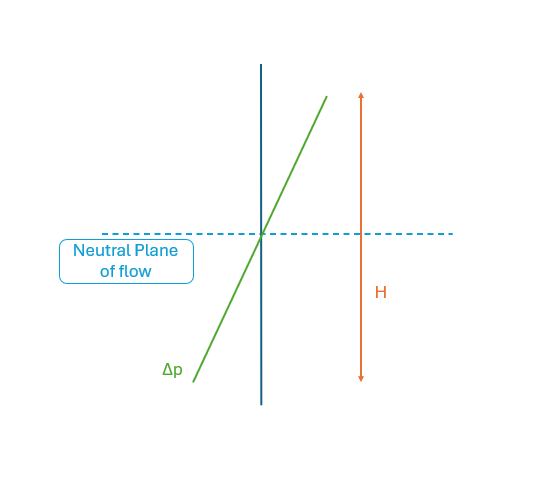
- The differential pressure vector profile is linear for Figure 4 due to the hydrostatic equation.
Additional information may be found in the ASHRAE Smoke Control Handbook, Appendix A, Fig. A1 (Handbook of Smoke Control Engineering 2024).
CONTAM Theory
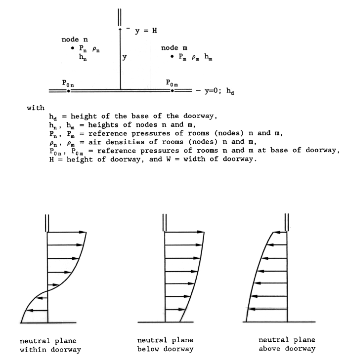
Figure 5 is from the public NIST document detailing AIRNET. It is identified as Figure Four in the CONTAM technical reference (Walton 1989).
Methods
| Method | Supported in Ventus | Supported in ContamW | Supported in CFAST | Supported in Pyrosim |
|---|---|---|---|---|
| One Opening Numerical Integration | Yes (2025.1 and later) | Yes | No | No |
| Two Opening Approximation | Yes (2025.1 and later) | Yes | No | No |
| Division into Directional Flow Areas | No | No | Yes | No |
One Opening Numerical Integration
In Ventus, users can calculate bidirectional flow with the Two-way - One Opening Flow Element as in Figure 2.
This is identical to the Single Opening Model with 2-way Flow in ContamW.
Two Opening Approximation
In Ventus, users can approximate the bidirectional flow with two openings offset from the neutral plane of the opening with the Two-way - Two Opening Flow Element as in Figure 3.
This is identical to Two Opening Model with 2-way Flow in ContamW.
Each opening will be set at a vertical distance of \(2/9 * H\) from the center of the opening.
See the Ventus User Manual section.
Each flow element will account for pressure drop due to opening height (local hydrostatic effect) and other (usually more significant) forces such as fan and building-scale stack effect.
Division into Directional Flow Areas
A fire-specific multi-Zone model like CFAST divides the pressure profile into up to 10 directional flow areas, or "slabs". Visit nist.gov/cfast for more information.
CFAST splits each compartment (Zone) into one upper layer and one lower layer. The flow can be characterized through calculation of the combination of each Zone. Put into practice, a colorful visual representation of an example compartment fire (NearFldDoor.smv) emerges. See Figure 6.
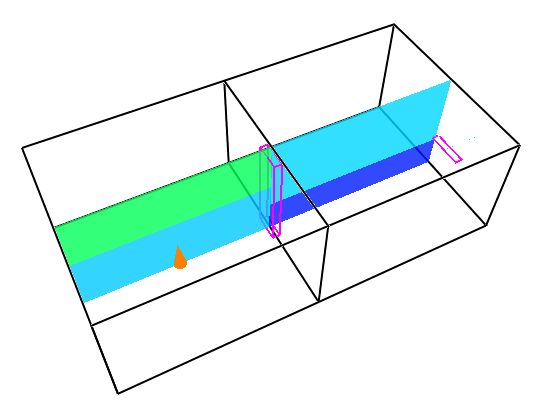
The temperature difference in layers can be visualized by comparing the color of each in Figure 6. For compartment fires in the real world, a visible smoke layer forms near the fire (see this FSRI experiment: living room fire showing smoke layer).
For modeling purposes, a large building can be divided into two fields: the near-field is near the fire, and the far-field is the rest of the building (Handbook of Smoke Control Engineering 2024)
Most modern standards argue that near-fire spaces should be modeled with calculations from at least two temperature Zones (upper layer and lower layer) per compartment. (“Fire Safety in Buildings - Smoke Management Guidelines” 2018) In Ventus and ContamW, the temperature and pressure are simplified to one "lumped parameter" per compartment, making it difficult to accurately model near-field flow (Handbook of Smoke Control Engineering 2024).
Example: Tall Window Between Zones
Model a mid-height window between Zones in Ventus. This provides the starting point for comparing one-way and two-way flow models in Ventus.
One-way Flow Simulation
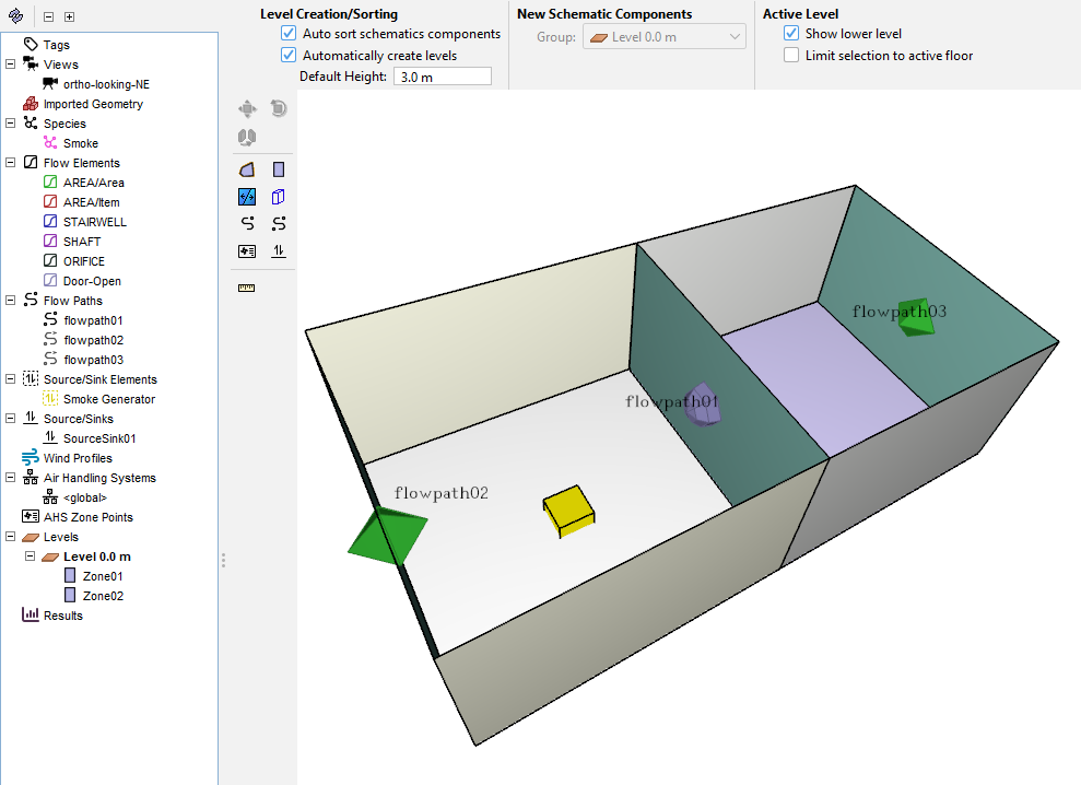
In this section, modify the 2-zone-contaminant.vnts model in Figure 7.
- Open
2-zone-contaminant.vnts. - Rename the East Zone, "Zone01" to "1" and the West Zone, "Zone02" to "2".
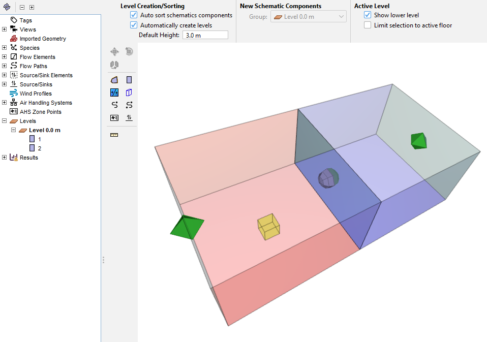
- Apply a temperature setting to 1 that forces a constant air temperature of 30 °C. This is well above the default Zone temperature of 20.0 °C; we can expect that varying density will create a pressure differential across the door.
- In the Property Panel, select the Color field to assign Zone 1 color to red and 2 to blue to visually distinguish hot and cold. Your model should now look like Figure 8.
- Double-click on the Flow Elements group in the Object tree to open the Edit Flow Elements dialog.
- Create a
Window-OpenFlow Element: - Duplicate the Door-Open Flow Element and rename it
Window-Open. An Orifice Area Flow Element with the following properties is appropriate:- Cross-Sectional Area of 1.25 m
- Flow Exponent of 0.5
- \(C_d\) of 0.78
- The default Reynolds number value.
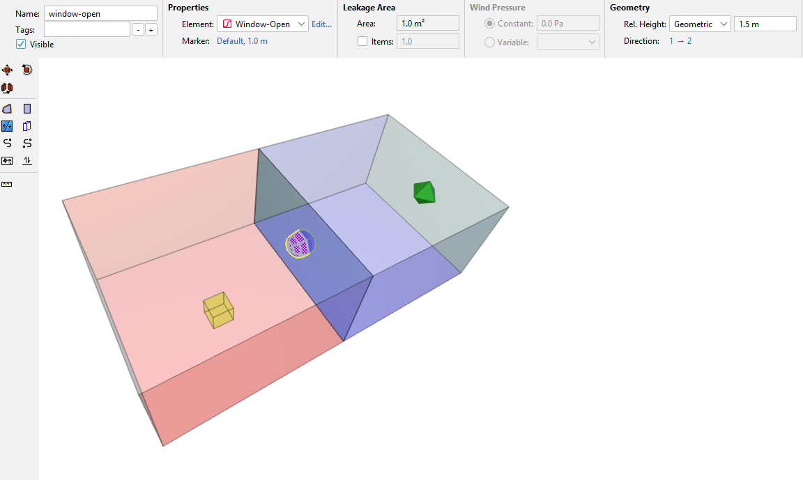
- Select the Flow Path between 1 and 2.
- Change the Flow Element type to
Window Open. - Change the Flow Path name to window-open.
- Check that the relative height is Geometric, 1.5 m.
- Delete the Flow Path between 1 and Ambient. Leave the Flow Path between 2 and Ambient; Zone 1 is only connected to Ambient through Zone 2 now. Your model should now look like Figure 9.
- Save the model.
- Open Analysis › Simulation Parameters.
- In the Time tab, check that the airflow simulation method and contaminant simulation method are both Transient.
- Set the simulation time to
100 swith a time step of1.0 s. - In the Simulator tab, select the
Vary density with time stepoption box to turn it on with max iterations per time step set to100. - Select OK to close the dialog.
- In the File menu, click
 Run Simulation.
One-way Flow Results
Open Path Data and expand the filters to show all data. All flow paths are zero for all times. There is no temperature-driven circulation of flow as expected in Figure 2.
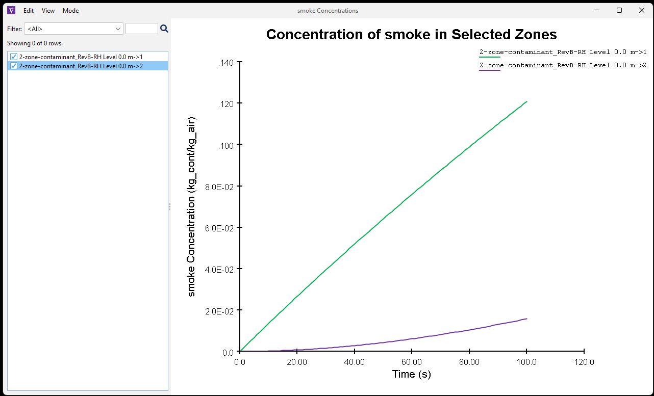
Get a quick visualization of contaminant transport through the native Ventus 2D Plot Tool as in Figure 10.
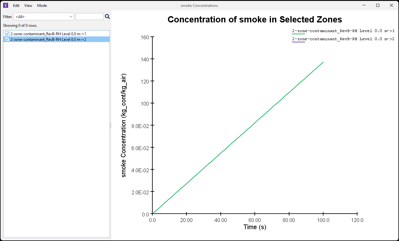
The contaminant is contained entirely in Zone 1.
Because the one-way flow path provides the only connection between Zones (and there is zero external pressure), there is no pressure differential and therefore zero flow. This is the net flow through the window – but it doesn’t account for air leaving Zone 1 and returning from Zone 2 across the vertical height of the opening. To track contaminant transport, bidirectional flow should be quantified.
Two-way Flow Simulation
Next, create a Two-way Flow simulation to track the bidirectional transport into and out of 1.
- Open the Edit Flow Elements dialog.
- Add the Flow Element:
- Duplicate
Window-Openand rename itWindow-Two-way. - Change the Model to
Two-way - One Opening. - Enter a Height of 1.25 m
- Enter a Width of 1.0 m
- Leave \(C_d\) as 0.78
- Duplicate
- Select OK to close the dialog.
- Edit the Flow Path window-open between 1 and 2:
- Change the Flow Element type to
Window-Two-way. - Rename the flow path window-open-two-way.
- Change the Rel. Height mode to Custom.
- Change the Rel. Height value to 0 m. As mentioned in the User Manual, the Custom property is appropriate for Two-Way Flow model Flow Path objects.
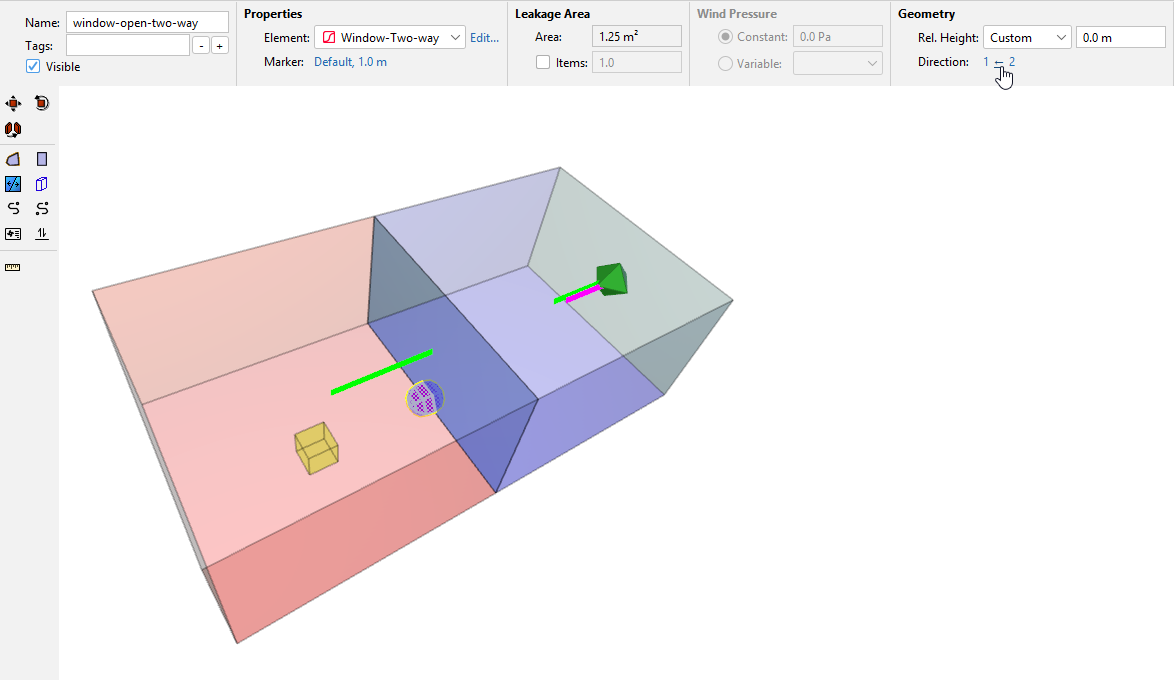
- Change the direction of positive flow in the property panel from
1 → 2to2 → 1. We expect that the flow will go this direction and set the sign convention accordingly, as in Figure 11.
- Change the Flow Element type to
- Save the model.
- In the File menu, click Run Simulation.
Two-way Flow Results
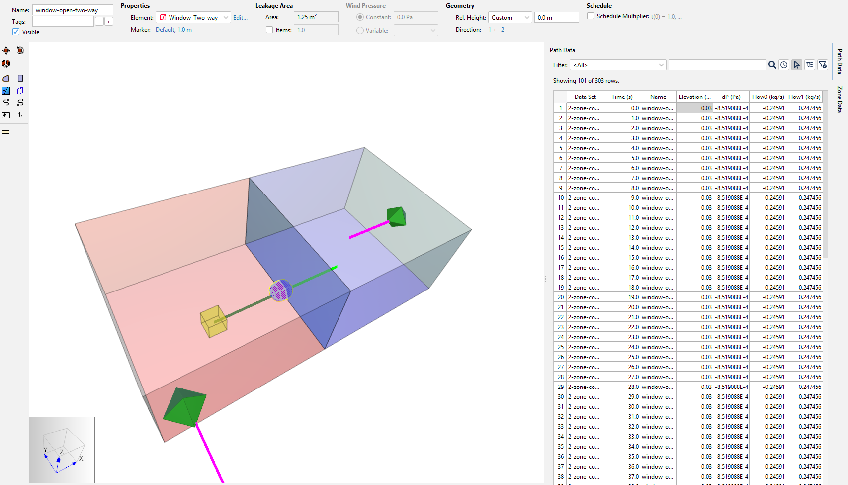
Open Path Data and expand the filters to show data. Now, there is temperature-driven circulation.
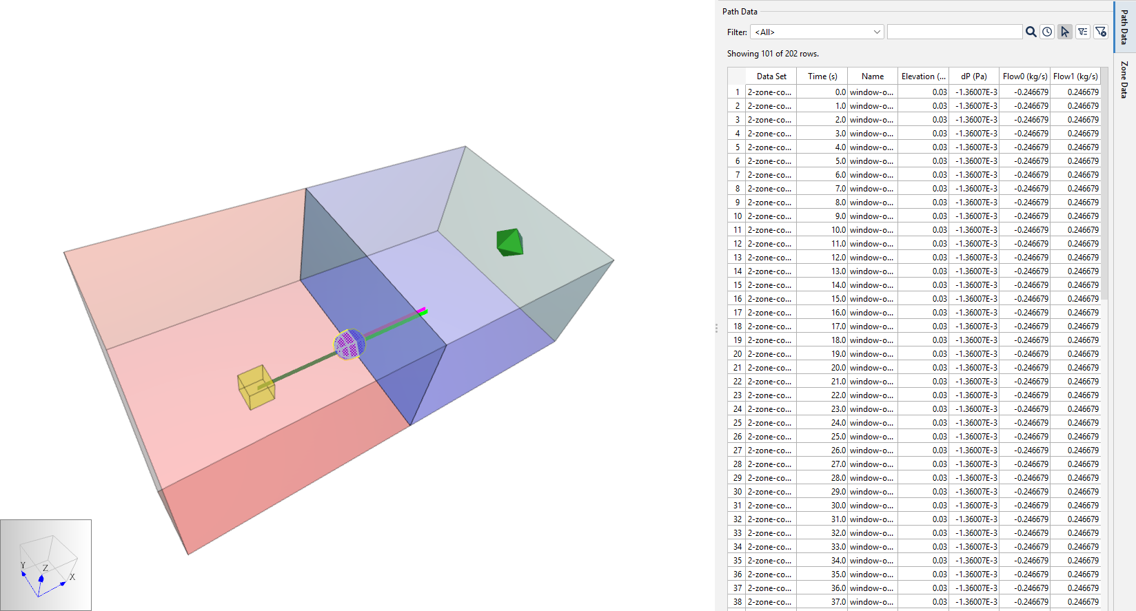
As in Figure 12, the sum of flow0 and flow1 add up a net flow of zero.
Also, the pressure differential is 0.00136 Pa in each direction.
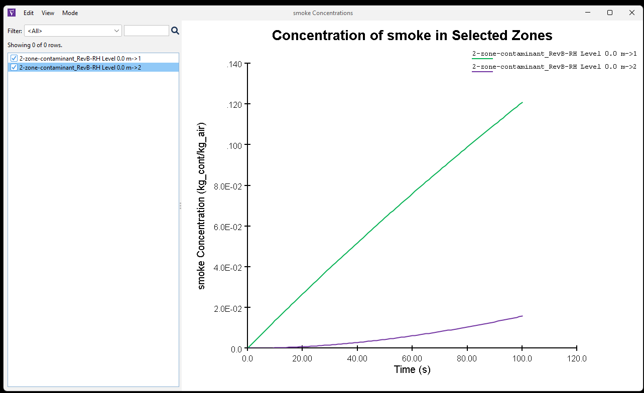
Get another quick visualization through the native Ventus 2D Plot Tool as in Figure 13.
This contaminant concentration data makes more sense.
When you introduce contaminants to a Ventus model with a significant horizontal temperature gradient, a two-way flow model can account for mass transport across the vertical opening.
Introduce External Pressure
Most smoke management systems will involve significant external pressures such as wind and stack effect (“Fire Safety in Buildings - Smoke Management Guidelines” 2018). These external pressures will reposition the neutral plane from mid-height of the opening and create net flow in one direction (See Figure 5).
Define an external pressure with Wind:
- Select the Flow Path on the East wall of Zone 2.
- In the Property panel, in the Wind Pressure tab, select Constant Wind Pressure and enter 0.00136 Pa. This is the magnitude of the driving pressure for each two-way flow.
- Add a Flow Path connecting Zone 1 to the Ambient Zone.
- Save the model.
- In the File menu, click Run Simulation.
Results with external pressures
Open Path Data and expand the filters to show data.
As in Figure 14, the sum of flow0 and flow1 add up a net flow of 0.001546 kg/s (not zero).
The external wind pressure repositions the neutral plane to create net flow in one direction, equivalent to both AREA/Area Flow Path magnitudes.
Get another quick visualization through the native Ventus 2D Plot Tool as in Figure 13.
The flow between Zones did not change enough to visually alter contaminant concentrations; Figure 13 and Figure 15 are nearly identical.
Conclusion
Key takeaways:
- Temperature differences and connections through tall vertical openings between zones can cause horizontal flow between those zones.
- When the flow neutral plane aligns within the height of a vertical opening, two-way flow modeling is necessary to account for mass transport of contaminants.
- In Ventus, Two-way Flow models assume uniform temperatures and concentrations throughout each Zone, making them a poor choice for near-field fire simulations.
- Flow Paths with Two-way Flow Elements are compatible with external pressure and stack effect models.
Additional information about two-way flow is included in:
- The ASHRAE Smoke Control Handbook, Appendix A (BIDIRECTIONAL FLOW)
- REHVA Guidebook No. 24, Fire Safety in Buildings - Smoke Management Guidelines, Annex 1 (PDS additional information)
- SFPE Handbook of Fire Protection Engineering, Performance-Based Design chapter, Figure 37.4 (Guidelines for substantiating a fire model for a given application)
To download the most recent version of Ventus, please visit the Ventus download page. Please contact support@thunderheadeng.com with any questions or feedback regarding our products or documentation.
Bibliography
“Fire Safety in Buildings - Smoke Management Guidelines.” 2018. Federation of European Heating, Ventilation and Air Conditioning Associations (FEHVA).
Handbook of Smoke Control Engineering. 2024. 2nd ed. ASHRAE, 180 Technology Parkway, Peachtree Corners, GA, USA: ASHRAE.
Dols, W. Stuart, and Brian J. Polidoro. 2020. NIST Technical Note 1887, CONTAM User Guide and Program Documentation, Version 3.4. Revision 1. National Institute of Standards and Technology, Gaithersburg, Maryland, USA: NIST.
Walton, George N. 1989. AIRNET - A Computer Program for Building Airflow Network Modeling. NIST, Gaithersburg, Maryland, USA: National Institute of Standards and Technology. https://www.nist.gov/system/files/documents/2018/03/16/airnet.pdf.
Related Tutorials
This Feature Demo details the steps to model basic Contaminants in Ventus.
This Feature Demo covers how to use the Performance Curve Flow Element
This Feature Demo details the steps to model door state changes in Ventus
Video tutorial demonstarting how to assign exit goals to percentages of the occupant population.
Tutorial demonstrating how to verify HVAC Pressure Drop in Pyrosim.
Tutorial demonstrating how to model a fire in Pyrosim.
How to simplify post-processing data collection with seasonal scenarios and scheduled stairwell temperatures.
This tutorial teaches the user how to perform a closed door Stairwell Pressurization study in Ventus.