 |  |
Overview
This tutorial is intended for Fire Protection Engineers (FPEs). We run a model with CFAST, use that data to calculate a Heat Release Rate (HRR) curve, and edit an existing Ventus model to model smoke transport. CFAST results data is provided; you do not need to run the simulation directly.
Learn how to simulate smoke transport throughout a simple six-floor condominium building; combine key Ventus features to simulate a transient smoke scenario and compare results to visual tenability requirements.
Before Starting
Before beginning this tutorial:
- Download the smoke-scenario.zip folder to follow along. The ZIP folder contains this tutorial’s starting files, solution files, and other tools.
- Understand how to: use Two-way Flow Elements, model Door States, and model Contaminants.
- Understand the concept of visibility and obscuration; this tutorial uses the mass optical density approach to correlate visibility with fuel concentration (See Visibility Calculation).
- Understand how CFAST simulates fire variables.
CFAST is a two-layer Zone fire modeling tool which uses airflow, heat transfer, and combustion differential equations. Visit nist.gov/cfast for a free download and more information. Unlike PyroSim, CFAST is a Zone model streamlined to define fire spaces in two layers; it generates a smaller amount of raw data which is easily input to Ventus. CFAST has been validated with test data for near-field fire simulation.
- Understand near-field fire modeling theory.
For modeling purposes, a large building can be divided into two fields: the near-field (close to the fire), and the far-field (the rest of the building). Most modern standards argue that near-fire spaces should be modeled with calculations from at least two temperature Zones (upper layer and lower layer) per compartment. In Ventus and ContamW, the temperature and pressure are simplified to one "lumped parameter" per compartment, making it difficult to accurately model near-field flow. (Handbook of Smoke Control Engineering 2024), (“Fire Safety in Buildings - Smoke Management Guidelines” 2018)
Additionally, the ideal gas law and fluid mechanics are especially important to understand when modeling smoke transport.
Introduction
In this tutorial, you will follow along to simulate smoke transport from a fast-growing (t2) fire in apartment Unit 1 (Level 2, 9.0 ft) with Ventus.
This example is inspired by the ASHRAE Handbook of Smoke Control Engineering, first edition. Chapter 19, Tenability Analysis and CONTAM, provides guidance for smoke control analysis. (Handbook of Smoke Control Engineering 2012)
Near-field CFAST fire simulation outputs (included in the Starting Point subfolder of the ZIP) are used to characterize Ventus inputs. Build on the model from Ventus Validation #3 and analyze tenability over 20 minutes. Tenability is determined by the maximum allowable concentration of soot, 3.26x10⁻⁵ lb/ft3 (5.18x10⁻⁴ kg/m3) (Handbook of Smoke Control Engineering 2012).
Fire Scenario Inputs
Defining the "fire"
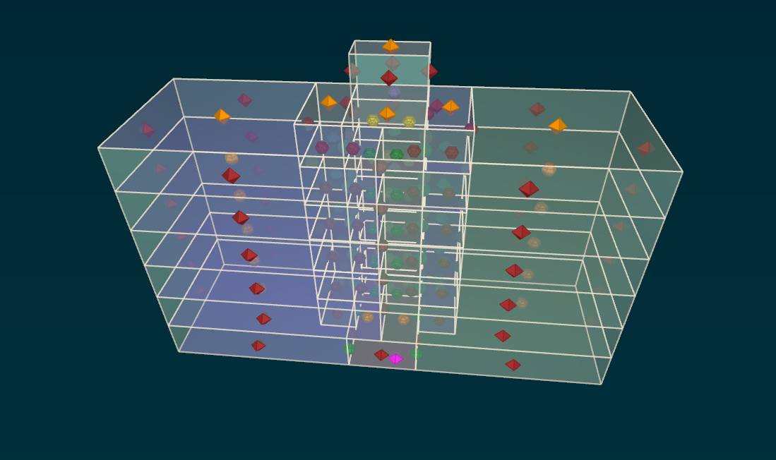
This scenario features a "fire" in Unit 1 of the six-floor condominium building in Figure 1:
- The fire is a fast-growing t2 fire with a maximum Heat Release Rate (HRR) of 2000 Btu/s (2110 kW) and a maximum fuel rate of 0.264 lb/s (0.120 kg/s). The fire reaches its peak at 213 s, and the peak duration extends indefinitely.
- The fuel is flexible polyurethane foam in horizontal configuration, with a chemical heat of combustion of 7,570 Btu/lb (17,600 kJ/kg). The mass optical density for polyurethane fuel is 1600 ft2/lb (0.33 m2/g), as in smoke control handbook Table 6.4 (Handbook of Smoke Control Engineering 2024). These values correlate the visibility effects to the amount of fuel burned without performing combustion stoichiometry (soot yield is accounted for implicitly in the correlation).
- Sprinklers are considered inoperable for this simulation.
Temperature Ventus Inputs From CFAST Output Data
After consulting the smoke control handbook, page 463, two Zones, Unit 1 and hall on Level 2, should be considered near-field (Handbook of Smoke Control Engineering 2024).
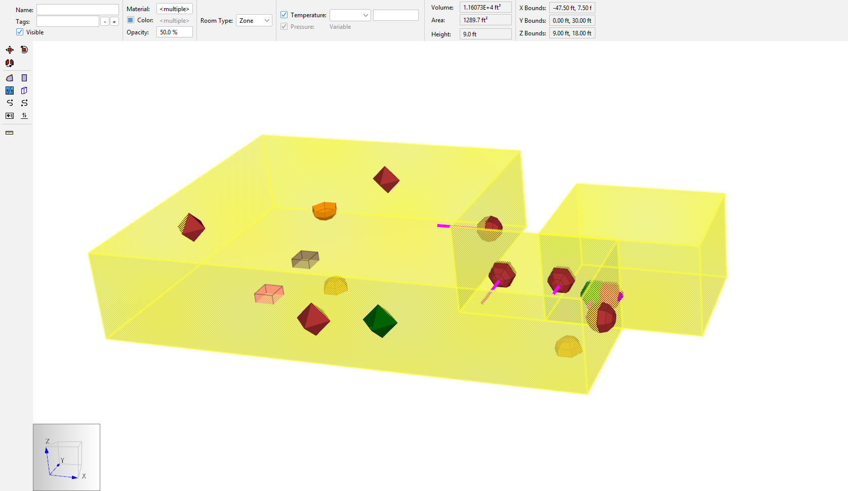
- Compartment geometry must be identical to near-field Ventus Zone and Flow Path data as filtered in Figure 3.
- CFAST fire curve input data should match the fire scenario geometry in Ventus.
(See the
CFAST Fire Propertiessheet of thesmoke-scenario-results-processing.xlsxfile from the Starting Point subfolder in the ZIP from this tutorial’s Overview section.) - Full details on inputs and methods appear in CFAST Method.
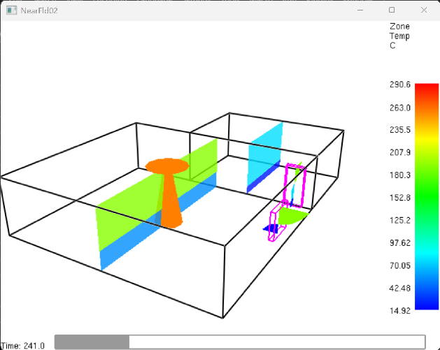
- A colorful visual representation of the fire (NearFld02.smv) appears in the Smokeview application as shown in Figure 2 from this tutorial’s Overview section.
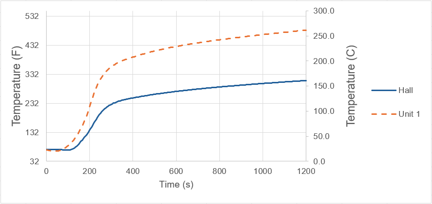
- From CFAST, the "compartment" temperature data is output with the
NearFld02_compartments.csvfile, providing data for the Unit 1 Zone and hall Zone. Compute one average Zone temperature from the CFAST compartment (two-layer) temperature information. This calculation is performed in theT_av-calcsheet of thesmoke-scenario-results-processing.xlsxfile from the zip folder; technical details are presented in section Tav Calculation.
| Time (s) | Unit 1 T_av, °F (°C) | hall T_av, °F (°C) |
|---|---|---|
| 0 | 73 (23) | 73 (23) |
| 60 | 71 (22) | 73 (23) |
| 120 | 103 (40) | 74 (23) |
| 180 | 185 (85) | 119 (48) |
| 215 | 264 (129) | 157 (70) |
| 300 | 371 (188) | 229 (109) |
| 600 | 444 (229) | 273 (134) |
| 900 | 478 (248) | 294 (146) |
| 1200 | 503 (261) | 310 (155) |
Fuel Generation Rate Ventus Inputs From Thunderhead HRR Calculator
We can model some parameters of a t2 file with a spreadsheet by Thunderhead Engineering: hrr-calculator_t2-growth-decay-v2.xlsm (in zip folder).
The fire t2 curve input matches the CFAST FastFire Fire properties in NearFld02.in for 0 < t < 1200 s.
Our sheet will provide simplified curve values of fuel generation rate to copy into the Ventus schedules.
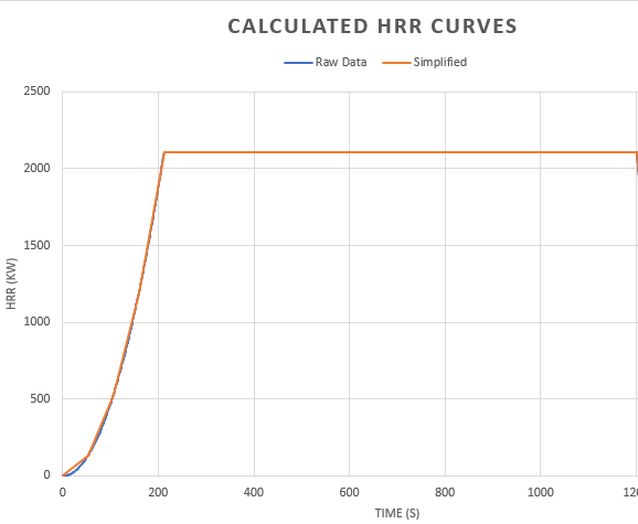
Ventus input data requires all the mass generated by the fire to create concentrations of fuel, soot, and other contaminants. The HRR spreadsheet is an efficient source of data for the total fuel mass released by the fire at each time
| Time (s) | HRR, Btu (kW) | Fuel Rate, lb/s (kg/s) | Fuel Rate Multiplier |
|---|---|---|---|
| 0 | 0 | 0 | 0 |
| 53 | 12.49 (131.7) | 0.0165 (0.00749) | 0.062 |
| 106 | 49.95 (527.0) | 0.0660 (0.0299) | 0.250 |
| 159 | 112.4 (1186) | 0.146 (0.0674) | 0.562 |
| 212 | 199.8 (2108) | 0.264 (0.120) | 0.999 |
| 213 | 2000 (2110) | 0.264 (0.120) | 1.0 |
| 1200 | 2000 (2110) | 0.264 (0.120) | 1.0 |
As in Table 2, the fuel rate is proportional to the fire’s HRR, with the maximum fuel rate defined in the Introduction.
Next, use temperature data in Table 1 to schedule Zone temperatures and the fuel rate data in Table 2 to schedule Species generation.
Model
Figure 1 in Overview is the starting point model from Ventus Validation #3, included in the zip folder.
In this section, modify the starting-model.vnts model with the fire scenario details.
- Unit 1 has an open window on the South wall that is 4.2 ft (1.28 m) wide by 4 ft (1.22 m) high with a sill 3 ft (0.914 m) above the floor. The window should have a discharge coefficient of 0.70, and two-way flow is expected.
- The door between Unit 1 and the hall opens at time t=60 s and remains open for the remainder of the simulation. The doorway measures 3 ft (0.914 m) wide by 6.7 ft (2.042 m) high, with a discharge coefficient of 0.75. Again, two-way flow is expected.
- The building temperature is 73°F (22.8 °C), and the outdoor temperature is –4 °F (–20 °C) with no wind. Atmospheric pressure is 14.3 psi (98.6 kPa) and relative humidity can be ignored.
- The stairwells, temperature controlled to 8 °F (-13 °C), each contain AHS supply units providing 2500 SCFM (1.42 kg/s).
- The temperature of Unit 1 and the hall change according to the schedule in Table 1.
After extracting the zipped files:
- In the folder smoke-scenario-starting-point open the starting file starting-model.vnts.
- Units for this tutorial should be US Customary (EN) units as shown in the File toolbar.
- Avoid confusion by renaming key Zones:
- Set
Level 2as the active level. - Rename the Zone of Unit 1 on
Level 2from Zone04_1 to Unit 1. - Also rename the Zone of the hallway on
Level 2from Zone00_1 to hall. - Set
Level 3as the active level. - Rename the Zone above Unit 1 from Zone04_1__1 to Unit 3.
- Set
Create new Flow Elements
Two new Flow Elements need to be added to the model to simulate the transport of smoke near the smoke source. The new Flow Elements are large holes best described with the Two-way Flow - Single Opening model (Handbook of Smoke Control Engineering 2012).
- In the Object Tree, double-click on Flow Elements to open the Edit Flow Elements dialog.
- In the dialogue, select New….
- Create two new
Two-way - One Openingmodel Flow Elements with the values in Table 3.
| Description | Name | Height | Width | Discharge Coefficient |
|---|---|---|---|---|
| Window, open | Window-O | 4.0 ft | 4.2 ft | 0.75 |
| Single Door, open | Door-SO | 6.7 ft | 3 ft | 0.70 |
- Choose green as the color for
Window-Oto follow along with this demo and select Apply. - Choose pink as the color for
Door-SOto follow along with this demo and select Apply.
Update the Unit 1 - hall door Flow Path
Edit the door between Unit 1 and hall on Level 2 to model closed and open situations.
- On the second level, select the
DOOR-SCtype Flow Path between Unit 1 and hall , flowpath42. - Rename this Flow Path unit-door-closed.
- Edit the Rel. Height to half of the door height, Geometric, 3.35 ft.
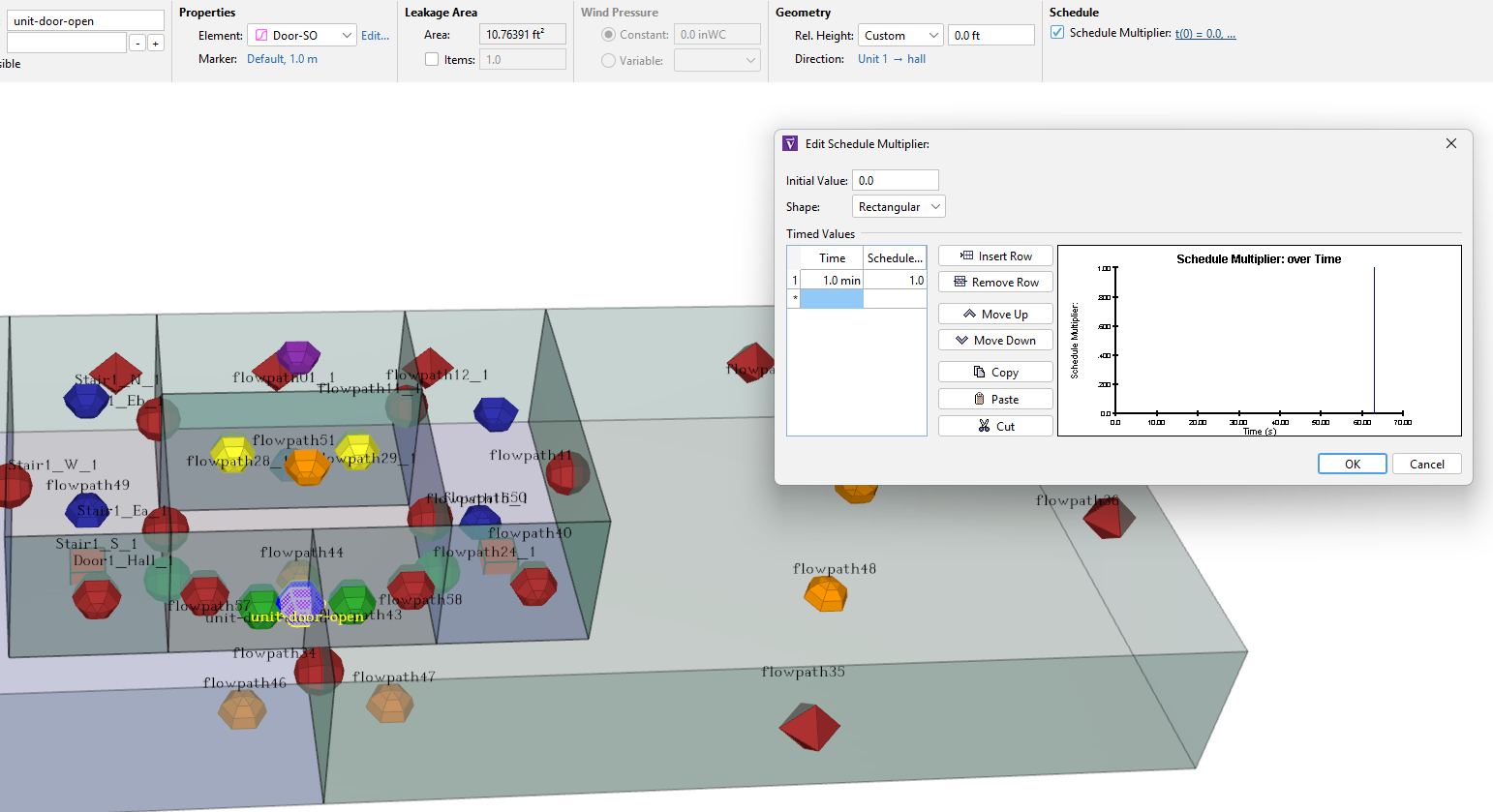
- Create a second Flow Path at the same location, of the type of flow element to
Door-SO. The path icon color should be pink. - Select the new Flow Path with the
Door-SOElement:- Rename this Flow Path unit-door-open
- Change the Rel. Height mode to Custom.
- Enter a Custom relative height value of 0.0 ft. For Two-way Flow Elements, to calculate accurate stack effect, each Flow Path Rel. Height should be input as sill/threshold height, not the center of the opening; for doorways this demands the usage of the Custom Relative Height mode (see the User Manual).
- Press ENTER. As mentioned in the User Manual, the Rel. Height value is clamped to the middle 98 % of the walls on which the endpoints are attached. In this case, the value becomes 0.09 ft (0.03 m). This is OK for our low-fidelity simulation.
- Create a door airflow on/off schedule for both Flow Paths so that the closed door leakage turns off at 60 s and the open door turns on at 60 s, as in Figure 6 and Figure 7.
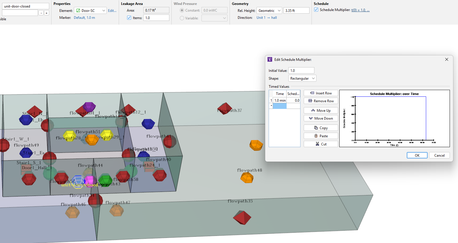 |  |
Create the window Flow Path
On the second level, create a new Flow Path between Unit 1 and AMBIENT.
- In the ribbon, select the
Window-OFlow Element. - The Flow Path icon color should be green.
- Rename this Flow Path window.
- Enter the Rel. Height as the sill height, 3 ft (0.914 m). (This relative height property is best in Geometric mode.)
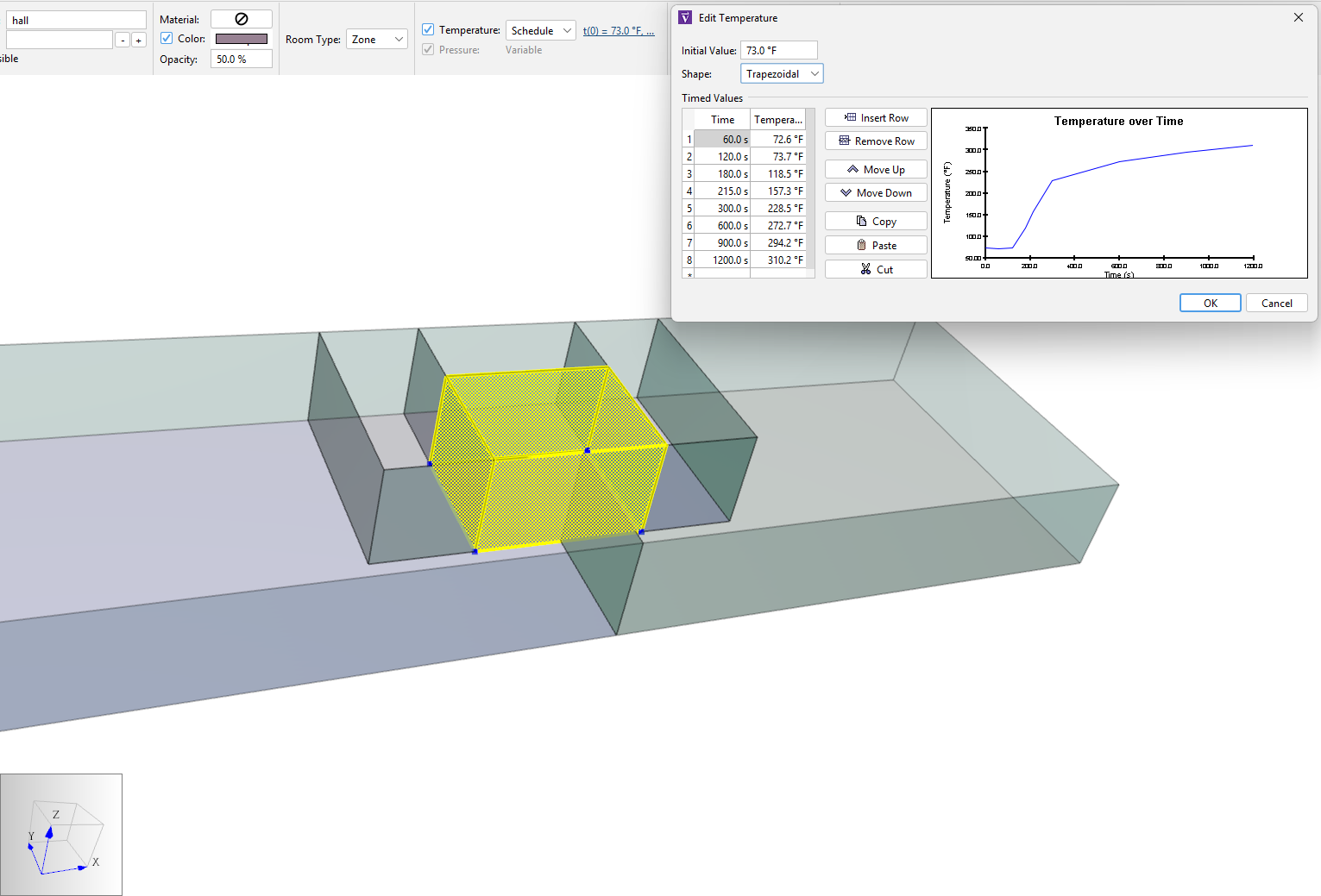
Create the Near-Fire Zone Temperature Effects
The heating of Unit 1 and the hall on Level 2 is modeled in Ventus with temperature schedules in Unit 1 and hall.
- The average temperatures in Table 1 should be imposed on these Zones.
- Use a Trapezoidal shape for both Unit 1 and the hall to achieve the desired temperature ramping in these Zones.
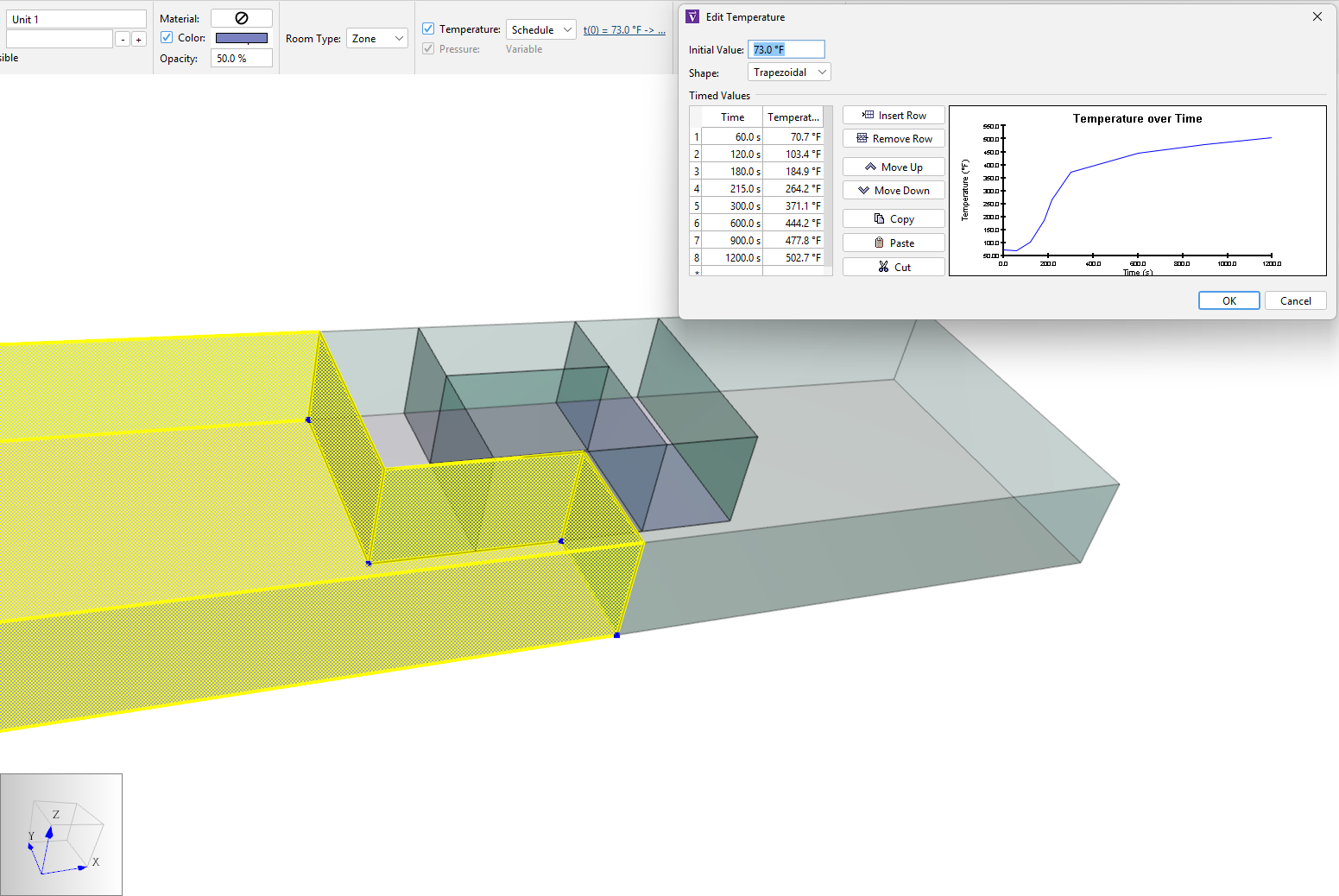 |  |
Define the contaminant
Next, create a contaminant study.
The "fire" will generate fuel in our Ventus simulation.
Create Fuel Objects
Define this contaminant as a Species so that we can calculate the concentration over time, in every Zone of the model.
- In the Object Tree, double-click on Species to open the Edit Species dialog.
- Click New… and enter the name
fuel, then press ENTER. - In the Edit Species dialog, enter the Description
polyurethane foam, horizontal configuration. - Enter 1 g/Mol for the molar mass of the soot.
Because
fuelis a trace contaminant, the Molar Mass will not matter in this simulation.
- Select Trace Contaminant per the smoke handbook guidance. In Ventus, "trace contaminants" are assumed NOT to impact the density of the air in the Zone due to their relatively small concentrations.
- Leave the default concentration set to 0.
- Click OK or press ENTER.
Create Source Elements
- In the Object Tree, double-click on Source/Sink Elements to open the Edit Source/Sink Elements dialog.
- Click New… and enter the name
fuel-gen, then click OK or press ENTER. - Use the Constant Coefficient model with species
fuel. - Enter a Generation Rate of 0.264 lb/s (0.120 kg/s). This is the peak fuel generation rate for the fire in Unit 1, as calculated in the HRR sheet and presented in Table 2 from Fire Scenario Inputs.
Place the Source
In Unit 1, define a source:
- Select add a source/sink from the draw sidebar.
The tool should automatically select the
fuelelement species. - Click to place the source anywhere in Unit 1. The source object will automatically appear in the 3D workspace with a Rel. Height of 0 ft, which is fine.
- Rename the source
source-1.
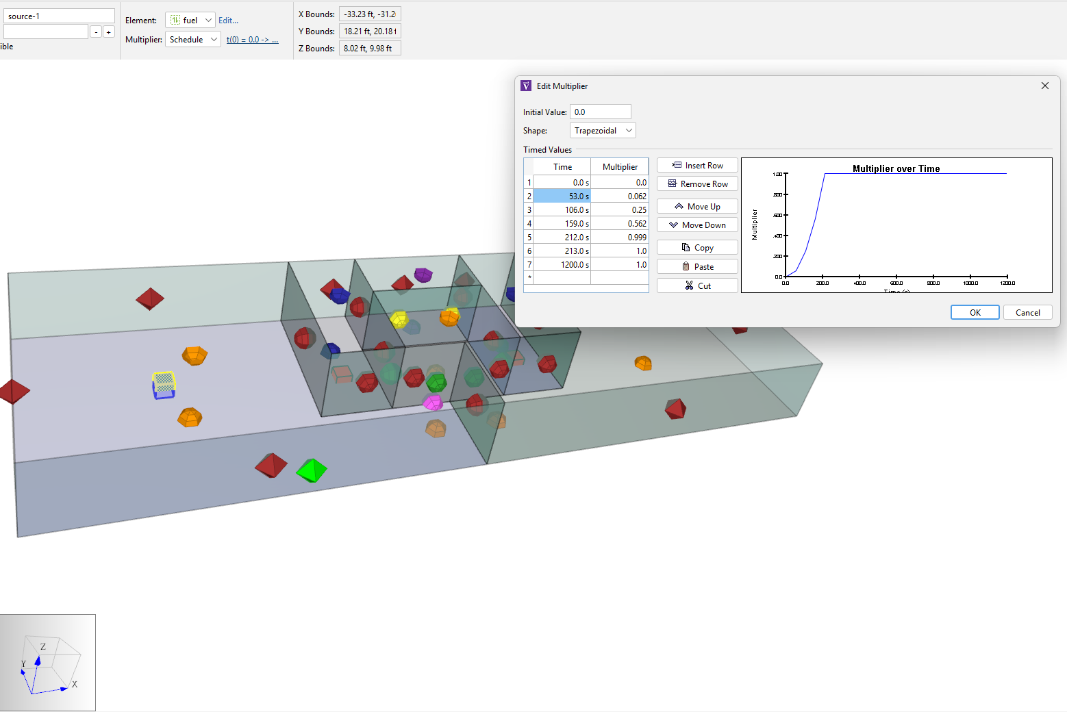
Schedule the Source
- Select source-1 object
- In the Property panel, change the Multiplier to
Schedule. - Edit the multiplier schedule.
- Enter a normalized Factor from Table 2.
The schedule for
Fcan also be copied from theSchedulessheet ofsmoke-scenario-results-processing.xlsx. The Ventus multiplier schedule dialog should look like Figure 10.
Fuel will be created in Unit 1 on Level 2 as desired.
Because the temperature of this Zone is also set to increase following Figure 4, ContamX will simulate changes in air density that may drive smoke flow through the building.
Additionally, the door to Unit 1 will open at 60 s.
Having accounted for the Flow Paths, temperature schedules, door opening, and contaminants, we are ready to configure the simulation.
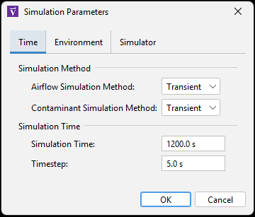
Simulation
Run a 20-minute simulation:
- Open Analysis › Simulation Parameters.
- In the Time tab, set the airflow simulation method and contaminant simulation method to Transient.
- Set the simulation time to 1200 s (
20 min) with a time step of5.0 s.
- In the Simulator tab, select the
Vary density with time stepbox to turn it on with the [default] max value of20iterations per time step. - Select OK to close the dialog.
- In the File menu, click
 Run Simulation.
Results
There is a set of calculated values for each time step (5 s) from 0 s to 1200 s. After running the model, Ventus automatically displays results with a playback menu below the Model workspace.
View Results in the 2D/3D workspace
- Use the playback menu to jump to a specific time, or watch the sequential progression of the simulation. The most interesting results occur between t=60s and t=65s, when the door opens.
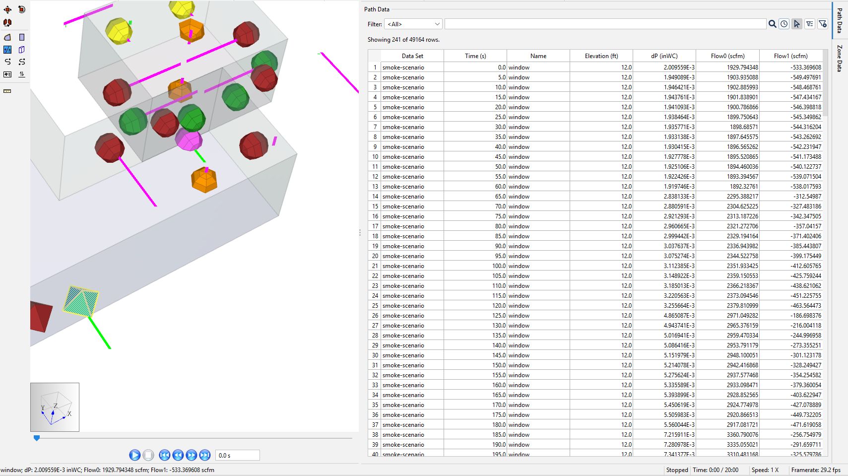
- Inspect the results at the window Two-way Flow Path for multiple time steps:
- In the workspace, select the window Flow Path.
- Open the Path Data Results panel.
- Select Filter to selected objects.
- De-select the Filter to current time step filter.
- Inspect the results at the unit-door-open Two-way Flow Path for multiple time steps.
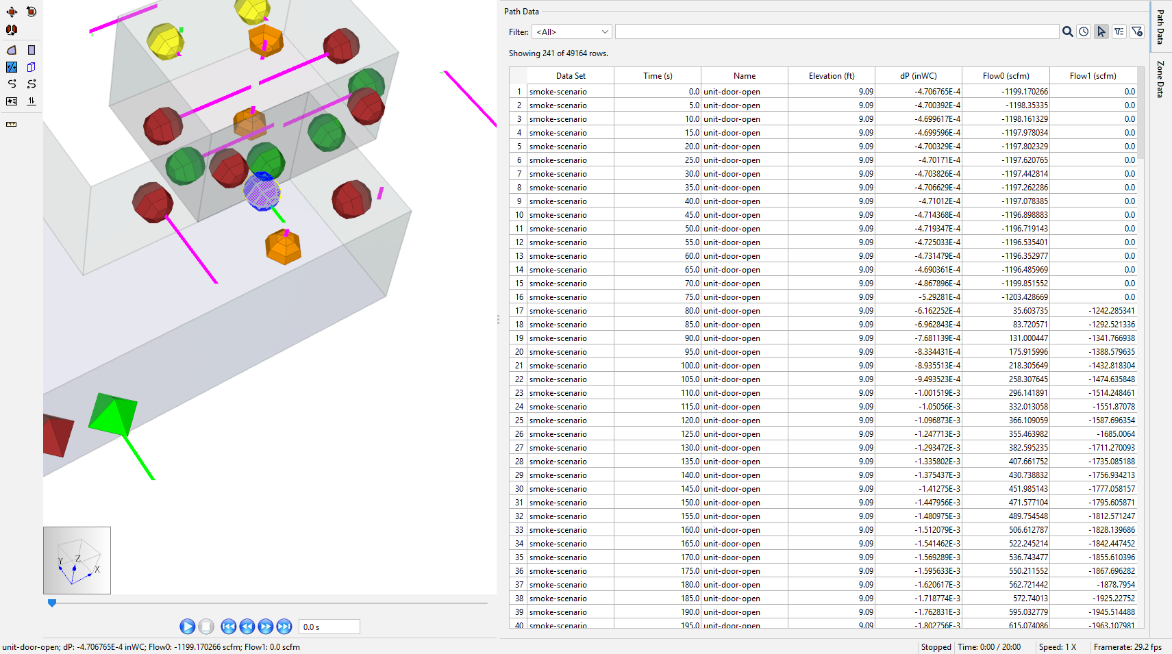
Two-way flow paths near the fire change the flow of smoke and toxins around the building, changing tenability results. There will be useful results in the Zone Data tab of the Results panel.
- Switch to the Zone Results panel.
- Select Filter to selected objects.

As in Figure 14, the Zone Data tab has:
- The temperature and density property for each Zone.
- The concentration of the contaminant,
fuel.
View Contaminant Results with the 2D Plot tool
Smoke obscuration (and tenability criteria) is correlated with fuel mass fraction.
Use the built-in 2D plot to quickly get a snapshot of key data:
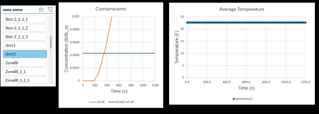
- Go to Results › Plot fuel Concentration.
- In the 2D Plot window, select the Unit 1, hall, and Unit 3 Zones. The tool generates and scales a plot of the concentration of fuel in the specified Zones over time in the window, as in Figure 15.
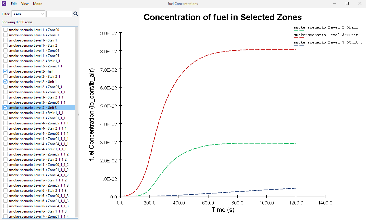
- Interpret the information:
- A concentration of greater than 7x10⁻² lb/lb is clearly exceeded in Unit 1 as plotted in Figure 15.
- A concentration of greater than 2x10⁻² lb/lb is clearly exceeded in the hall.
- From Introduction, the soot concentration corresponding with the visibility criterion is 3.26x10⁻⁵ lb/ft3 (5.18x10⁻⁴ kg/m3). This corresponds to a cutoff mass fraction of 4.30x10⁻⁴ lb/lb (kg/kg), using Standard Air.
- Therefore, Unit 1 and hall fail the visibility requirement within 20 minutes.
Next, examine the contaminant results in more detail.
Export results and post-process
Export all Zone Data (all Zones, all time steps):
- In the Zone Results panel, deselect Filter to selected objects.
- Use CTRL+A to select all the Zone Results data.
- Copy (CTRL+C) the table values into a spreadsheet tool.
Post-processing
Paste it into the Ventus-results sheet of the smoke-scenario-results-processing.xlsm file.
- Paste (CTRL+V) the data into the
Ventus-resultssheet. - Enter the cut-off mass fraction, 4.30x10⁻⁴ lb/lb (kg/kg). By entering visibility cut-off mass fractions, using table data filters, and scaling excel plots, you can examine every Zone for tenability over time on one screen.
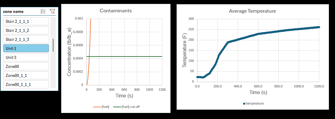
As in Figure 16, conditions become untenable after about 45 seconds.
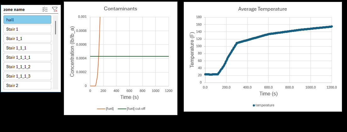
As in Figure 17, conditions become untenable after about 2 minutes.
As in Figure 18, conditions become untenable after about 5 minutes.
You can quickly run a version of the model where there are no fans pressurizing the stairs; stairwells would become smoky. Or, run a version where the fan size is increased to supply 3300 SCFM; the hall and Unit 3 would stay tenable.
Conclusion
The use of fans (AHS Supply Points) in the stairwells is revealed to be an effective strategy to protect the building overall. Air from the stairwells produces a low level of pressurization in the lobbies relative to units This air also dilutes what smoke leaks into the lobbies. These mechanisms work together to reduce smoke movement in the building.
You should now be familiar with how to model complex smoke transport scenarios and the process to export results quickly. Through thoughtful use of the tools provided in Ventus, you can scope complex tenability scenarios and iterate airflow system design to meet multiple objectives.
To download the most recent version of Ventus, please visit the Ventus Download page. Please contact support@thunderheadeng.com with any questions or feedback regarding our products or documentation.
Acknowledgements
The author of this tutorial would like to thank Stuart Dols at the US National Institute of Standards and Technology for his helpful and rapid responses that were needed to properly construct the ContamW model of this complicated simulation.
Appendix
Visibility Calculation
The soot in smoke reduces visibility of an egress route for occupants in an emergency situation. Visibility (\(S\)) is the distance that an observer can identify an object relative to the background, measured in length units. Minimum visibility distance is often used as an Egress tenability requirement. By making some conservative assumptions about line-of-sight distances and types of emergency signs, fire protection engineers can estimate a threshold visibility requirement for a building. In this tutorial, we use the mass optical density approach to correlate visibility with polyurethane soot mass optical density.
The Mass Optical Density Approach:
Mass optical density characterizes how easily certain frequencies of light can penetrate a substance. Optical density (\(δ\)) is determined through experiments of fuel burn and recorded percent obscuration (\(λ\)). The mass optical density (\(δ_m\)) is effectively normalized from optical density (\(δ\)) with mass concentration.
\(δ\) quantifies the probability of light impacting components of this particular solute in an air solution rather than passing through it as coverage (length squared) per amount of material (mass).
\(δ_m\) is material-dependent based on the particulate composition of products of combustion. The value is linked to a fuel for easier reference and because typical fuels have typical byproducts.
EQ 6.17 from the smoke control handbook:
\(S = \dfrac{K}{2.303 δ_m m_f}\)
Where
- \(K\) is the proportionality constant for the egress route lighting conditions
- \(δ_m\) is the mass optical density for the substance, length2/mass
- \(m_f\) is the mass concentration of the fuel per volume of the mixture, mass/length3
(Handbook of Smoke Control Engineering 2024)
Per Example 19.7 instructions, assume that the occupants need to see 25 ft in all Zones, which is the requirement for the largest Zone in the building. (Handbook of Smoke Control Engineering 2012) In reality, small rooms would not require as high visibility; for example, the stairwells would be easy to navigate with only 15 ft visibility.
If S = 25 ft, \(δ_m\) = 1600 ft2/lb (0.33 m2/g) for flexible polyurethane, and K = 3 (minimum) from Table 6.3, the mass concentration of fuel must be limited to no more than \(m_f\) = 3.26 E-5 lb/ft3 (5.18 E-4 kg/m3).
Assuming a dry air density and CONTAM Standard Air, this corresponds to a cutoff mass fraction of 4.26x10⁻⁴ lb/lb (kg/kg).
(Calculations are done on the visibility-calc sheet.)
CFAST Method
To predict heating the space, the CFAST model should match Ventus as much as possible.
Fire
The fire is fuel-limited until t=213 s, then the fire is air-limited and sustains a HRR of 2110 kW.
(These specifications are determined by the first edition of the smoke handbook in Example 19.1, Part 2.)
This "unit fire" uses the FastFire settings from (1st edition) Example 18.1 Part 1, which builds on the Standard.in file (renamed User_Guide_Example.in and included with the current CFAST 7.7 download).
The only specifications that are different from Ex 19.1 Part 2 in CFAST are the inclusion of hall and the use of the Heskestad plume model.
Stairwell Pressurization
Static pressurization of the far-field stairwells will have some effect on the near-field compartments. This was not addressed in CFAST, and is a source of uncertainty.
Plume Model
The Heskestad plume entrainment model is now the only option for smoke entrainment calculations, heat transfer, and ceiling jet temperature modeling in CFAST.
See the SFPE Handbook of Fire Protection Engineering (2008) as well as discussions since then about best practices and conservative smoke modeling.
For more information, see: the CFAST discussion group discussion and a GitHub call heskestad_plume example.
(Richard D. Peacock and Reneke 2023)
Output
The results from CFAST that are used in the Ventus model were copied from NearFld02_compartments.csv and pasted into the T_av-calc sheet of smoke-scenario-results-processing.xlsx for reformatting and the Tav calculation.
Soot and CO concentrations are not input to Ventus.
Tav Calculation
The two Zone temperature data can be converted into a single Zone average using a weighted average approximation.
EQ 19.1 from the ASHRAE smoke control handbook:
\( T_av = \dfrac{T_u * (H - z) + T_l * z}{H}\)
where
- \(T_av\) is the weighted temperature average
- \(T_u\) is the upper layer temperature
- \(T_l\) is the lower layer temperature
- \(H\) is the Zone height
- \(z\) is the upper layer height
(Handbook of Smoke Control Engineering 2012)
In the T_av-calc sheet of smoke-scenario-results-processing.xlsx, the pasted CFAST outputs are converted and the Ventus T_av input is calculated.
(In reality the temperature experienced would depend on the height of the occupant as they move around the building.
Any evaluation of exposure to thermal radiation should consider the upper layer temperature and heat transfer.)
Flow Models
Flow parameters can be modeled in CFAST within a two-zone temperature profile (upper layer and lower layer). In Ventus and ContamW, the temperature and pressure are simplified to one lumped parameter per compartment, making it difficult to precisely model near-field flow.
Many network models however suffer from not having a detailed heat transfer analysis and often temperature profiles must be assumed, or they must be determined in separate programs and used as input to the smoke movement program. (Black 2010)
In CFAST
As in Figure 19, the opening ("vent") can be partitioned into as many as ten flow segments ("slabs") in CFAST to account for multiple boundaries and directions of flow. For simple compartment fires with standard air mixture, six is the maximum number of required slabs (CFAST, the Consolidated Model of Fire Growth and Smoke Transport 1993).
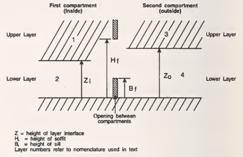
For each flow slab:
\(w = 2/3 (C) \sqrt{2 \rho} \times W \times (y_t - y_b) \dfrac{|ΔP_t|^{3/2} - |ΔP_b|^{3/2}}{|ΔP_t| - |ΔP_b|} \)
where
- \(C\) is the orifice coefficient of flow.
Use
0.70for the Window and0.75for the door as presented in Table 3. - \(ρ\) is gas density, taken from the "upwind" source compartment layer.
- \(ΔP_t\), and \(ΔP_b\) are the pressure differentials across the vent at the top and bottom of the slab respectively
- \(W\) is the cross-sectional width of the slab
- \(y_t\) and \(y_b\) are the height of the top and bottom of the slab respectively
(CFAST, the Consolidated Model of Fire Growth and Smoke Transport 1993)
If you look closely at the doorway Flow Path (vent) graphic while playing the NearFld02 results simulation in Smokeview, you can see the number of slabs and flow regime graphics changing as the fire develops like Figure 20 and Figure 21.
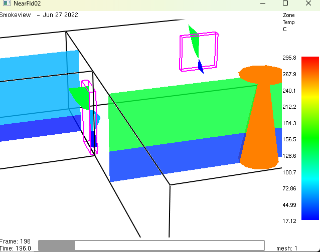
Breaking flow into subsections is particularly important when a compartment fire is under-developed (CFAST, the Consolidated Model of Fire Growth and Smoke Transport 1993).
For the door in Figure 20, the segments, in ascending height, are:
vent bottom→layer transitioncompartment2layer transitioncompartment2→layer transitioncompartment1layer transitioncompartment1→vent top.
Breaking flow into subsections is less important when the fire is fully-developed.
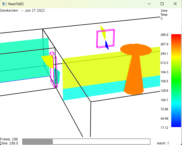
For the door in Figure 21 the segments are:
layer transitioncompartment2→layer transitioncompartment1layer transitioncompartment1→vent top.
vent bottom → layer transitioncompartment2 is negligible; the flow can be modeled with only two segments.
In Ventus and ContamW
ContamX network model calculations do not support division of flow into slabs.
By assuming that the air temperature in a Zone is constant throughout, the hydrostatic equation is used to relate pressures at various heights. The window and doorway can both be modeled as continuous openings with the Two-Way Flow Element described in Modeling Two-way Flow in Ventus.
Best Practice
The best practice for near-field smoke transport will depend on the problem. Additional information about Two-way Flow is included in:
- ASHRAE Smoke Control Handbook, Appendix A (BIDIRECTIONAL FLOW)
- REHVA Guidebook No. 24, Fire Safety in Buildings - Smoke Management Guidelines, Annex 1 (PDS additional information)
- SFPE Handbook of Fire Protection Engineering, Performance-Based Design chapter, Figure 37.4 (guidelines for substantiating a fire model for a given application)
Bibliography
CFAST, the Consolidated Model of Fire Growth and Smoke Transport. 1993. Building and Fire Research Laboratory, NIST, Gaithersburg, Maryland, USA: National Institute of Standards and Technology. https://doi.org/10.6028/NIST.tn.1299.
Handbook of Smoke Control Engineering. 2012. 1st ed. ASHRAE, 1791 Tullie Circle N.E., Atlanta, GA, USA: ASHRAE.
“Fire Safety in Buildings - Smoke Management Guidelines.” 2018. Federation of European Heating, Ventilation and Air Conditioning Associations (FEHVA).
Handbook of Smoke Control Engineering. 2024. 2nd ed. ASHRAE, 180 Technology Parkway, Peachtree Corners, GA, USA: ASHRAE.
Black, W.Z. 2010. “COSMO—Software for Designing Smoke Control Systems in High-Rise Buildings.” Fire Safety Journal 45. https://doi.org/10.1016/j.firesaf.2010.07.001.
Dols, W. Stuart, and Brian J. Polidoro. 2020. NIST Technical Note 1887, CONTAM User Guide and Program Documentation, Version 3.4. Revision 1. National Institute of Standards and Technology, Gaithersburg, Maryland, USA: NIST.
Richard D. Peacock, Glenn P. Forney, Kevin B. Mcgrattan, and Paul A. Reneke. 2023. CFAST Technical Reference Guide. NIST, Gaithersburg, Maryland, USA: National Institute of Standards and Technology. http://dx.doi.org/10.6028/NIST.TN.1889v1.
Related Tutorials
Modeling Contaminants
Reading Time: 7 minutes -
Contaminants
cad
flow
species
contaminants
transient
-
Contaminants
cad
flow
species
contaminants
transient
This Feature Demo details the steps to model basic Contaminants in Ventus.
Balancing Occupant Flow Through Multiple Doors
Reading Time: 1 minute -
venue
doors
flow
-
venue
doors
flow
Video tutorial demonstrating the difference in evacuation times when occupant flow is properly balanced.
Distribute Exit Goals
Reading Time: 1 minute
-
behavior
doors
flow
groups
profile
Video tutorial demonstarting how to assign exit goals to percentages of the occupant population.
Evacuation of Theatres and Stadiums
Reading Time: 1 minute
-
stadium
venue
behavior
doors
flow
groups
profile
Video tutorial demonstrating how to effectively simulate evacuation of theaters and stadiums using Pathfinder.
Modeling Two-way Flow
Reading Time: 11 minutes
-
flow
contaminants
transient
Learn when and how to model Two-way Flow in Ventus.
Modeling Fans: Performance Curves
Reading Time: 10 minutes
-
Doors
flow
schedules
transient
This Feature Demo covers how to use the Performance Curve Flow Element
Modeling Door States
Reading Time: 7 minutes
-
Doors
flow
schedules
transient
This Feature Demo details the steps to model door state changes in Ventus
Closed Door Studies
Reading Time: 6 minutes
-
smoke control
REHVA
cad
flow
This tutorial teaches the user how to perform a closed door Stairwell Pressurization study in Ventus.