2025.1 Seasonal Scenarios in Ventus

Introduction

This tutorial details the steps needed to:

Simulate multiple seasonal conditions with Scenarios in Ventus
Apply Zone temperature schedules in Ventus
Run a transient simulation of the proposed Pressure Differential System (PDS)
Quickly export key results and streamline data post-processing

Necessary files are in this zip folder: condo-seasonal-scenarios.zip.

Example Geometry

Use the steady-state winter model from the Ventus Validation #3 Tutorial. For information related to creating the Ventus starting model, as in Figure 1, see Ventus Validation #3 Tutorial.

You may assume total symmetry of the building, and only examine Unit 1 and Stair 1. In our model, the x-coordinate is measured along the east–west axis, the positive y-axis points north, and the z-coordinate measures height. Therefore, Unit 1 and Stair 1 are on the West side of the building.

Example Requirement

In this example, you are asked to examine the proposed PDS to meet one fictional mid-rise building requirement:

Pressure differentials on the doors connected to the stairwell must be between + 0.10 and + 0.35 inches water column (inWC), or + 25 to + 87 Pascal (Pa). A positive differential is defined from the stairwell to surrounding volumes.

Modify the file for a three-season simulation

Chose either English (US Customary, EN) or Metric (SI) units for your model. The starting model and this tutorial were made in English units.

Table 1. Temperature Scenarios for Ambient Weather.

Model Condition	Temperature ( °F)	Temperature ( °C)
Building	73	22
Winter	-4	-20
Isothermal	73	22
Summer	105	41

Open the file and confirm the following:

The design flow rate for each AHS Supply (on Level 2) is 2500 SCFM per supply. This is the fan rate for the proposed PDS. More information on Air Handling Systems (AHS) is available in the Ventus user manual.
In the Simulation Parameters menu, the Default Zone and Junction Temperature is set to 73 °F as in Table 1. This is a set point for the building’s thermostat.
In the Weather and Wind menu, Ambient Temperature is set to -4 °F, Relative Humidity set to 0 % RH, and Wind Speed is set to 0 ft/s.

Create Seasonal scenarios

To create a total of three scenarios:

In the Weather and Wind menu, use the edit command for Ambient Temperature.
Enter additional values from Table 1: 73 and 105 in degrees Fahrenheit (22 and 41 in degrees Celsius) and select OK. This will create multiple scenarios in Ventus and associated results folders to organize each set of results.
The other parameters remain appropriate.

Create Zone temperature schedules

Often, when modelling seasonal variation, unheated spaces like the stairwells are not controlled. It is necessary to simulate the stairwell temperatures to accurately predict stack effect and flow conditions. We can use the transient simulation settings in Table 2 to model conditions like stairwells within each scenario.

Table 2. Stairwell Temperatures for Each Scenario.

Model Condition	Stair Temperature ( °F)	Stair Temperature ( °C)	Schedule
Winter	8	-13	0 - 1 h
Isothermal	73	22	1 - 2 h
Summer	89	32	2 - 3 h

Create a temperature schedule for stairwell Zones:

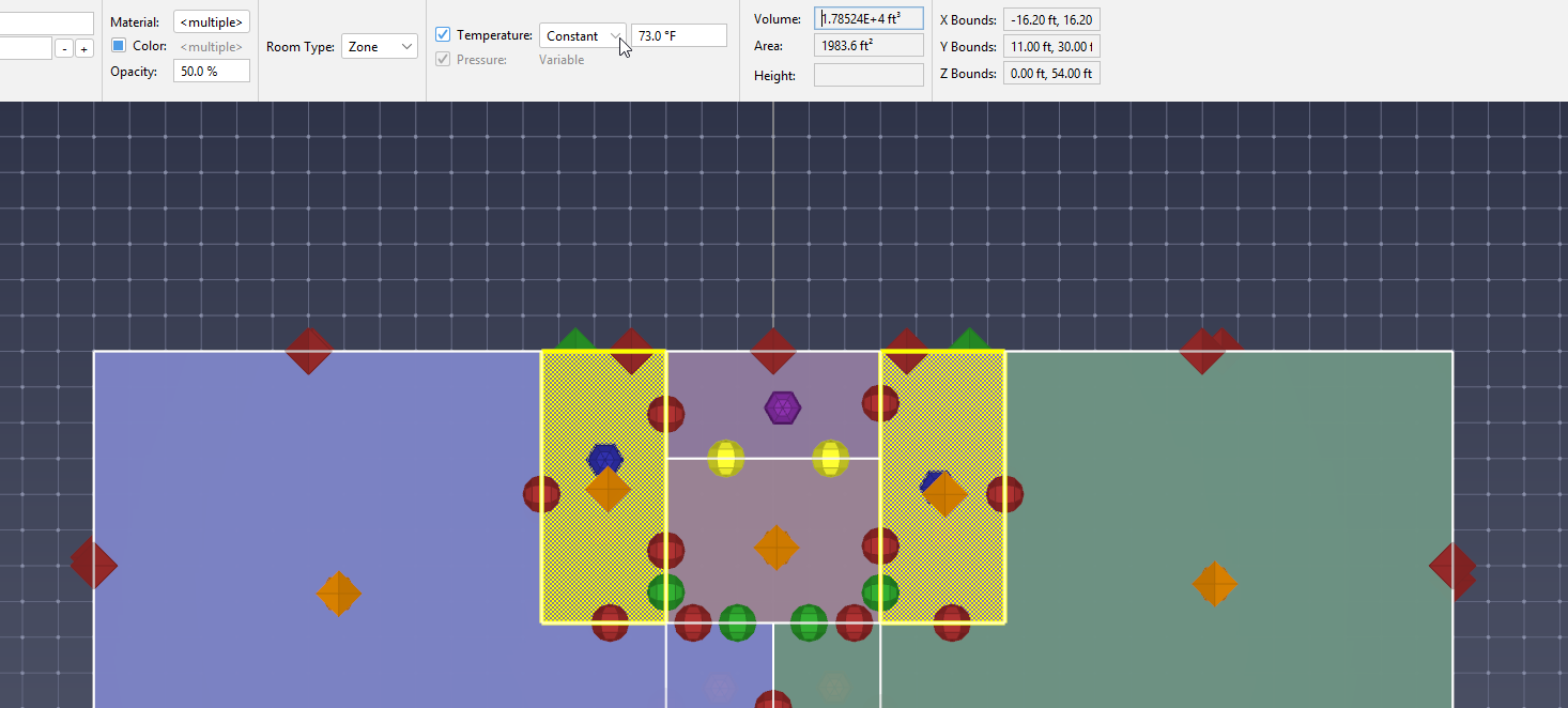
Select all stairwell Zones. Make sure to avoid selecting the stair Zones on Level 7, since the stair Zones on that level are Ceiling type areas above stairwell shafts. It may help to hide Flow Paths and AHS Zone points.
In the properties panel, toggle the temperature setting box. The Zone definition should change as in Figure 2 so you can select schedule in the drop-down menu. This will enable the schedule editor.

Turning temperature setting ON imposes a set condition onto the Zone so that the Zone will no longer be defined by the model’s default temperature.

Figure 2. Open the Zone temperature setting box to select a Zone temperature schedule.

Figure 3. Ventus stair Zone temperature schedule.

Input the schedule:

Select the hyperlinked schedule to open the schedule editor dialogue.
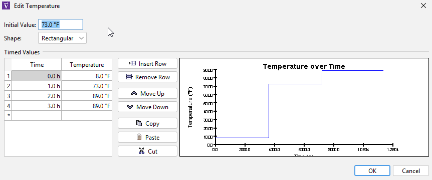
Leave the Function Shape as Rectangular.
Enter the stairwell temperature values in Table 2 for each hour of a three-hour simulation, so that the temperature plotted over time looks like Figure 3.
Close the schedule editor
In the Simulation Parameters menu, change the Airflow Simulation Method to Transient with a Simulation Time of 3 h and a Time Step of 30 min.
In the Simulation tab of the Simulation Parameters menu, ensure that the Vary density with time step setting is OFF. We do not want temperature changes in the stairwells to change airflow for our steady-state scenarios.

You can also copy/paste the schedule in table format from the Schedules sheet of the seasonal-scenarios.xlsx Excel file, included in the zip folder.

Putting it together

For each weather scenario, Ventus will run a 3 hour simulation and model the stair temperatures changing at 1 hour and 2 hours. Viable data is presented in Table 3

Table 3. Putting Together Scenario and Schedule Data.

Weather	Scenario Ambient Temperature	Stair Temperature	Simulation Time
Winter	-4 °F (-20 °C)	8 °F (-13 °C)	0-1 h
Isothermal	73 °F (22 °C)	73 °F (22 °C)	1-2 h
Summer	105 °F (41 °C)	89 °F (32 °C)	2-3 h

Weather

Scenario Ambient Temperature

Stair Temperature

Simulation Time

Winter

-4 °F (-20 °C)

8 °F (-13 °C)

0-1 h

Isothermal

73 °F (22 °C)

1-2 h

Summer

105 °F (41 °C)

89 °F (32 °C)

2-3 h

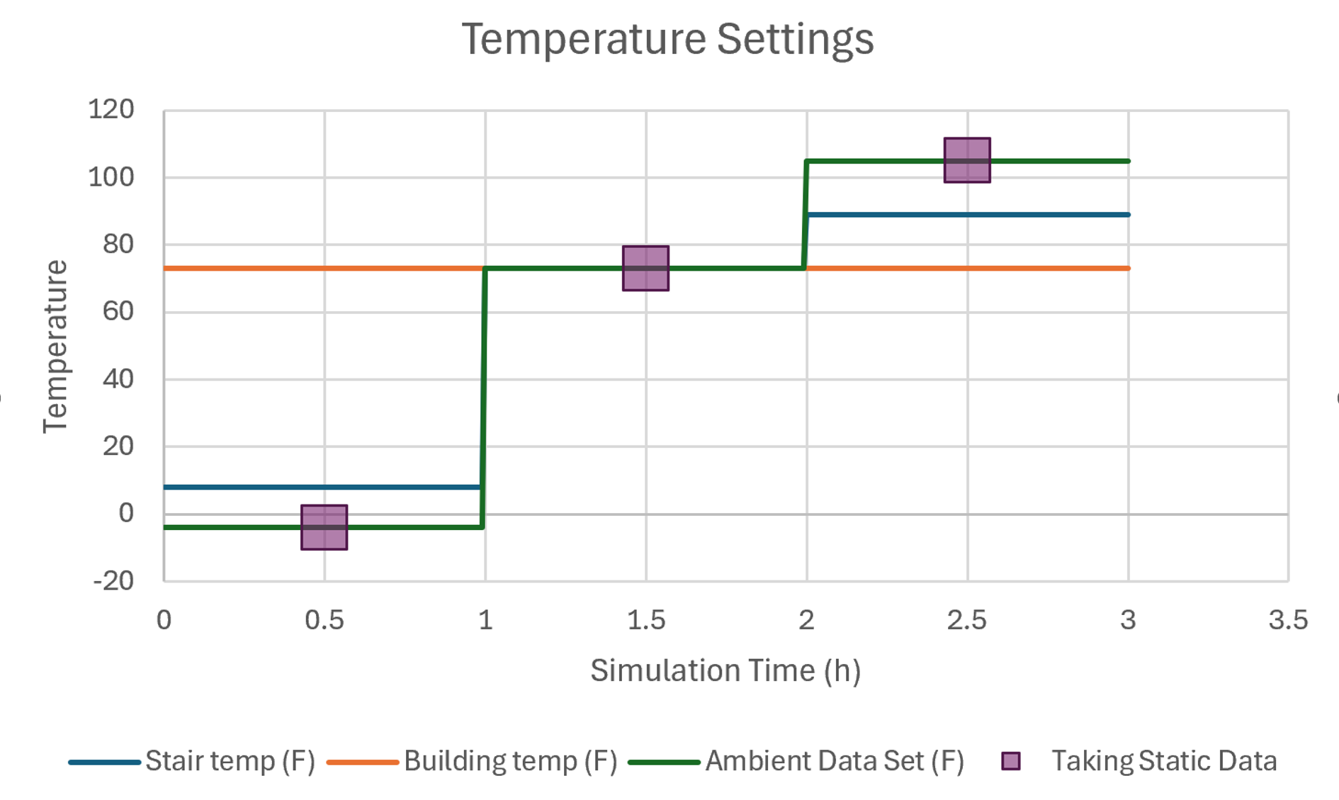
It would be mistaken to draw any conclusion from the 105 °F weather / 30 minute data, etc; we can only combine the stair Winter temperature setting with the Winter temperature weather.

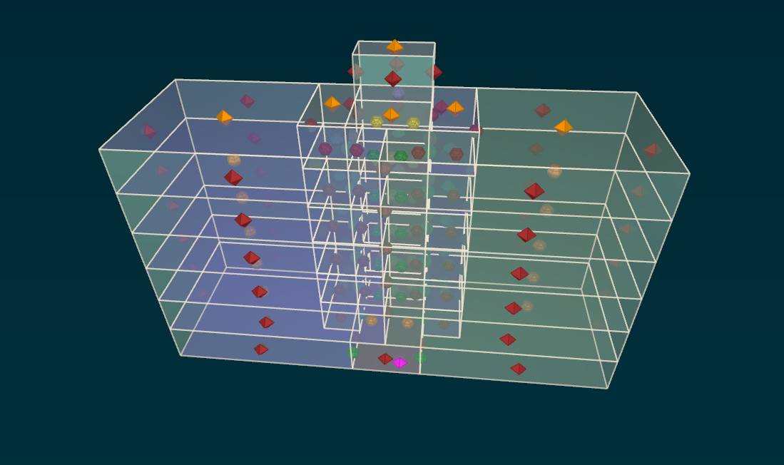
By changing the temperature of these Zones each hour and exporting data away from the model temperature changes, this model will be quasistatic. The model is solving airflow at each time step, without accounting for density variations between time steps. A visual representation of this method to create temperature differentials is presented in Figure 4. Quasitatic data can be taken at 30 min, 90 min, and 150 min.

Vis of method — Figure 4. Visualization of temperatures over time for the Ventus model.

Run the model

Immediately after running the model, the Ventus playback bar pops up on the bottom of the view window. Also, scenario folders appear in the results section of the Object tree.

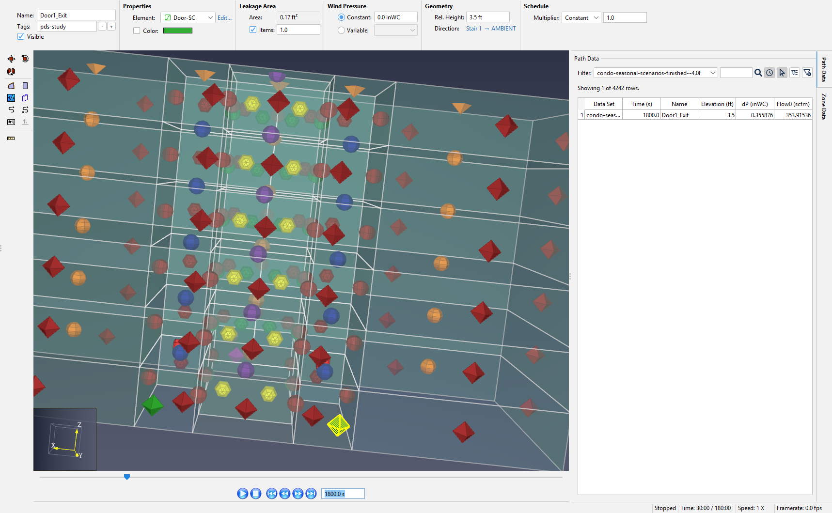
To investigate particular results, you can enter time into the playback bar and filter the scenario data as in Figure 5

vnts scrn view 3temps isolate door1 2025 1 — Figure 5. Examining the Stair 1 exit door results for the winter scenario.

Process Results

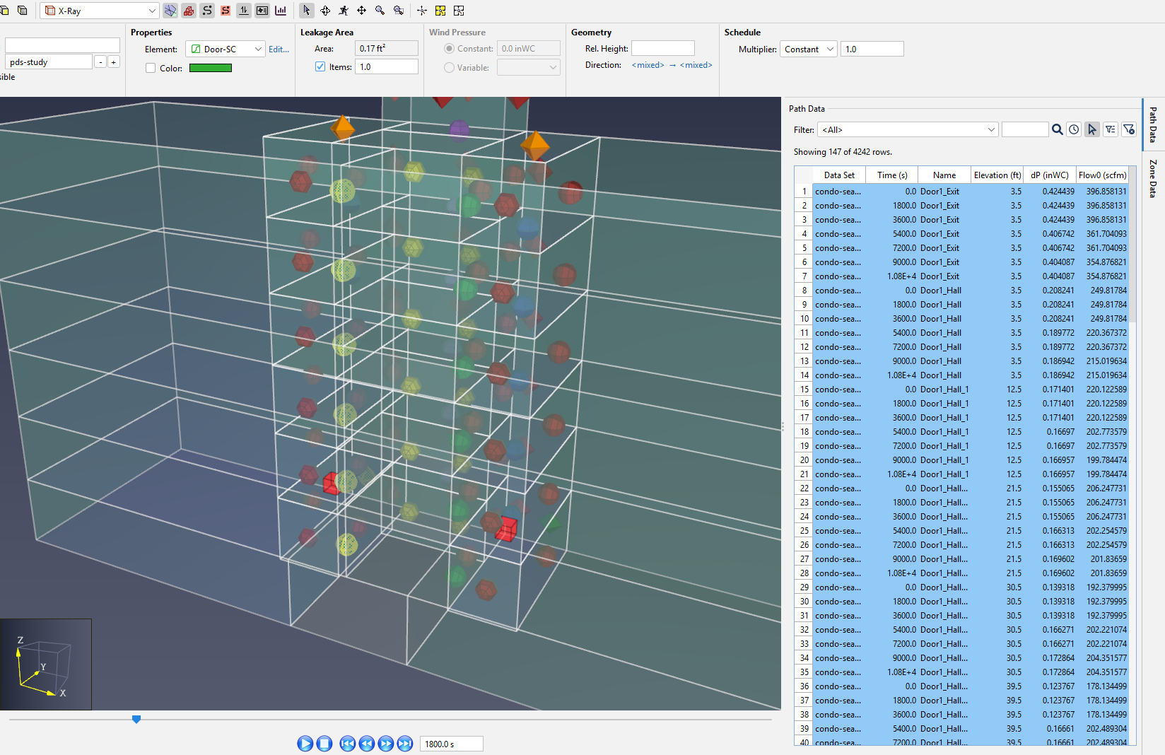
Open the results Path Data results panel, which contains a results table and filters.

To isolate relevant data:

In the 3D View window, use the CTRL key to quickly select all Stair 1 → door Flow Paths.
In the results panel, toggle the selection tool icon ON to filter only results associated with the selected objects.
Also, toggle the time step filter tool OFF to show all transient data.
Ensure that the scenarios filter is set to <All> data to show all seasonal data. The settings should match those in Figure 6.

Tips:
use CTRL+Z if you lose your selection group at any point.
tag the Flow Path group to efficiently select objects on multiple levels, per the user manual.

Figure 6. Filters for efficient data export and post-processing.

Export results

To transfer the data:

Use CTRL+A to select all and CTRL+C to copy the data.
Open the appropriate Excel workbook from the zip folder for your unit selection. In this demonstration, we open seasonal-scenarios-EN.xlsx.
After reading the release notes, switch to the sheet Ventus-results-table and paste the results data into the table.

You have now successfully exported the data.

Filter between scheduled Zones and weather data

It is important to isolate data between each scenario and the time-dependant stairwell temperatures. Remember that viable data is a combination of the seasonal scenario and the scheduled stair temperature in Figure 4. Use the Data slicers in Excel to isolate the appropriate data. For example, the data for the low temperature scenario can be filtered and analyzed as in Figure 7.

Compare criteria and simulation results

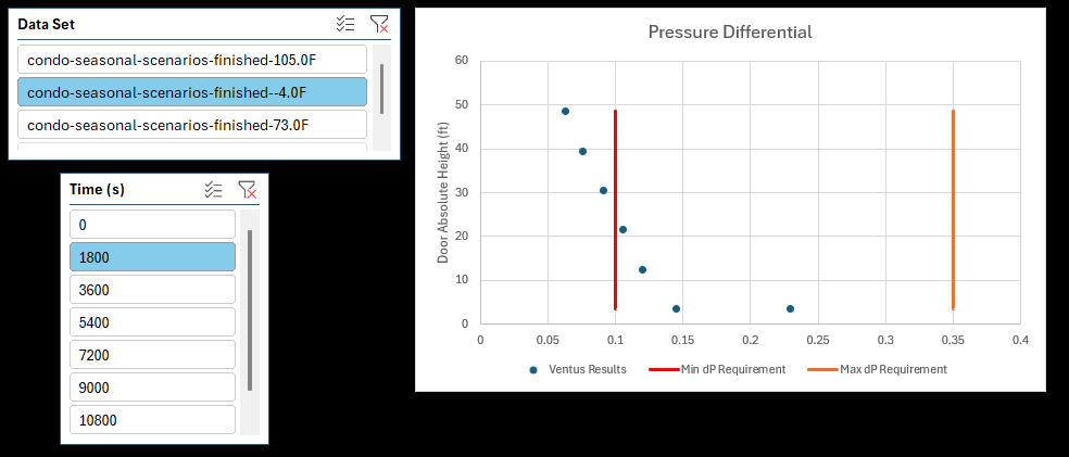
excel scrn view 3temps dP criteria not met 2025 1 — Figure 7. This pds fails to maintain the differential pressure requirement.

The pressure differential criteria are not met for this PDS design. We need to modify the stairwell pressurization by increasing the AHS Supply design flow rates.

If desired, you can export the results data from Ventus before changing the model.

In the toolbar, under Results select Show Link-Path Flows to dump data into your web browser.
From your browser, save the exported .html file something like seasonal-scenarios-2500scfm.

Change the model, and re-run the simulation

Iterate to improve the PDS:

On Level 2, or in the Object Tree, select both AHS supply objects.
Enter a Design Flow Rate of 3200 SCFM.
Select run, over-write previous results, and follow steps in Export results again to update the excel data.

Ventus scenarios and schedules enable you to update geometry once only, maintaining model data integrity. This avoids many headaches related to version control and file management.

Examine the new results.

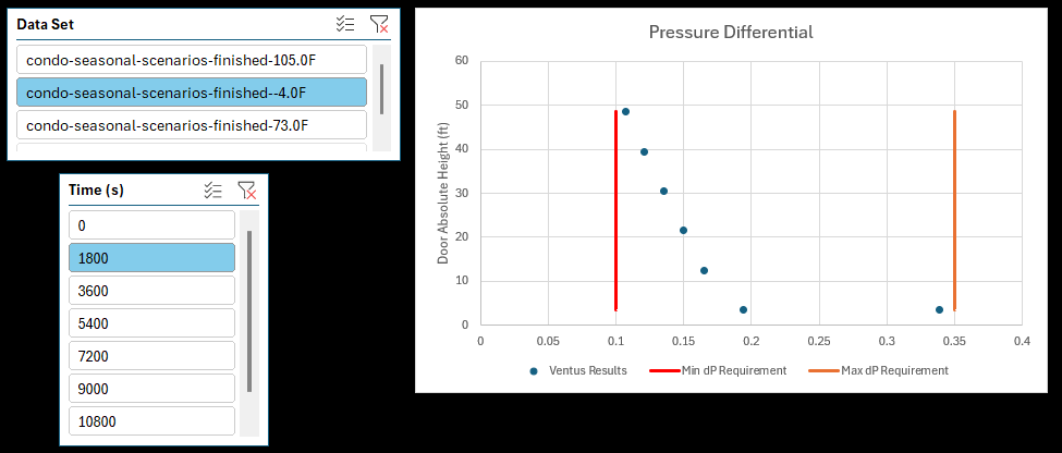
excel scrn view 3temps dP criteria met 2025 1 — Figure 8. This pds does maintain the differential pressure requirement.

If desired, you can export the results data and save it something like seasonal-scenarios-3200scfm.

Conclusion

This tutorial provides an example process to efficiently group scenarios in one Ventus model and maintain data integrity:

Seasonal scenarios with temperature schedules enable PDS iteration.
create your own plots, pressure differential requirements, and air flow evaluation as desired. Our spreadsheet represents a starting point for whatever workflow you follow.
Scenarios could be added to model varied wind conditions too.

To download the most recent version of Ventus, please visit the Ventus Download page. Please contact support@thunderheadeng.com with any questions or feedback regarding our products or documentation.

Seasonal Scenarios in Ventus