2025.1 Modeling Fans: Performance Curves

Overview

This tutorial is intended for users of Ventus that wish to model a fan with performance curve data. It will demonstrate how to use the Performance Curve Flow Element to model a simple fan Flow Path. This tutorial also explains "below Cut-off" fan operation and how the Cut-off ratio can be used to scale performance curves.

Before Starting

Before beginning this tutorial:

Download the Modeling Doors models to follow along.
Read through the Performance Curve Flow Element section in the User Manual.
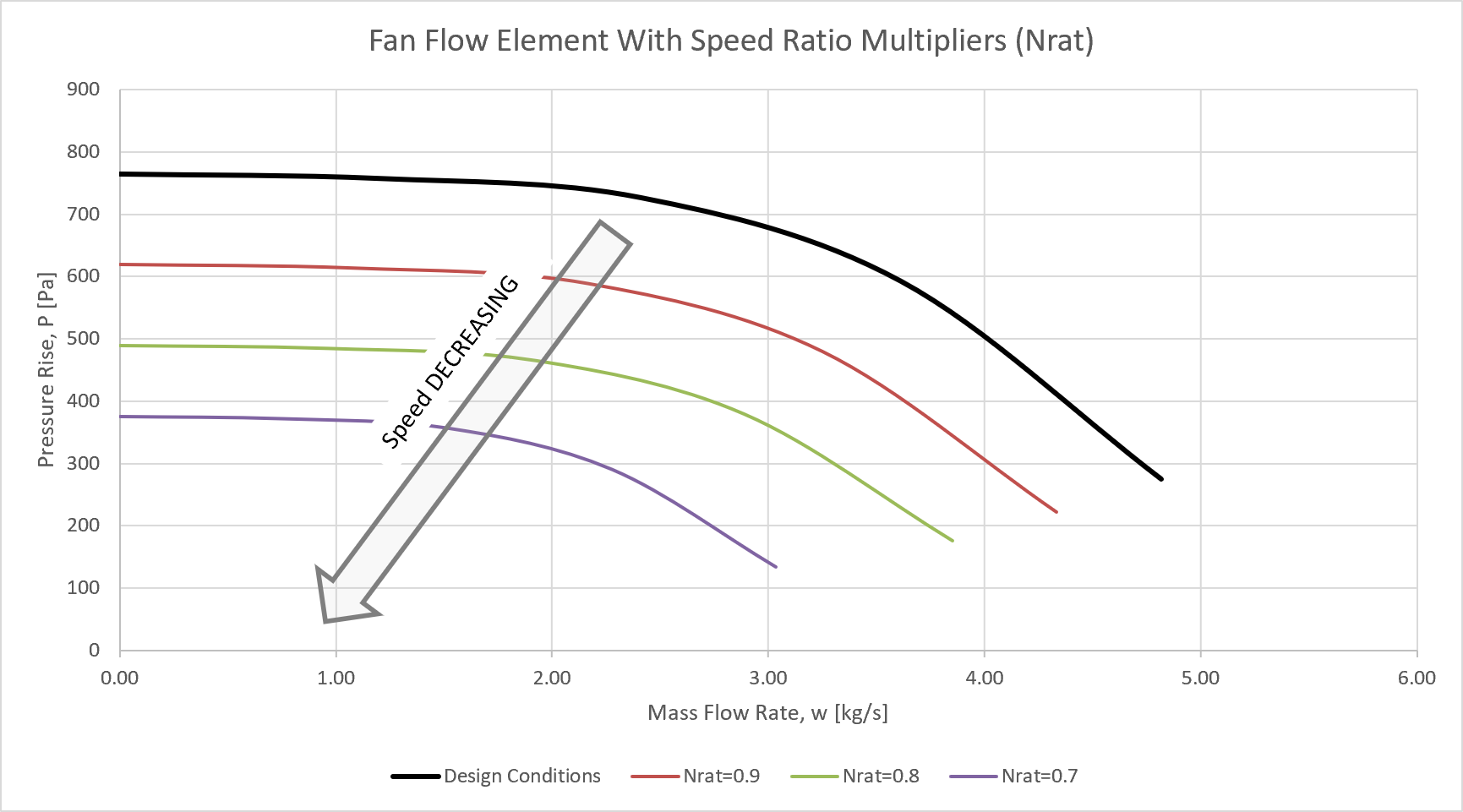
Understand the Fan Laws represented in Fan Laws with speed ratio, which is the plot shown in the above section of the User Manual.

Introduction

When modeling airflow systems in Ventus, it is often desired to compute fan (blower) operation points with performance Curve data for a given set of conditions. Traditionally, the performance curve must be matched with the system curve to obtain operating point of the selected fan. With Ventus, the operating point of the selected fan is computed automatically by ContamX.

Additionally, when fan systems turn off, users must account for the possibility of airflow through fan openings. Cut-off Conditions describe the opening flow model for each Performance Curve Flow Element.

To showcase the new Performance Curve Flow Element, we will use a simple two Zone model. This model is available in the modeling-doors-start.vnts file that you downloaded in the zip folder above. Each Zone in the model has a pre-modeled wall leakage Flow Path on one of its exterior walls, and Zone00, the West Zone, has a 1000 SCFM AHS Supply to pressurize the model.

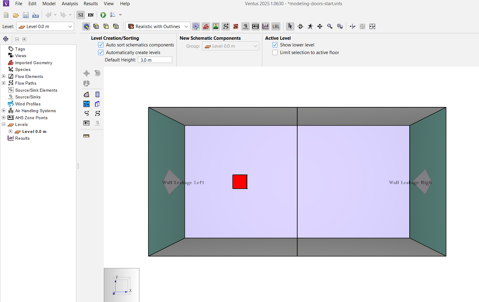
This model is also configured to use the Transient Simulation method to analyze non-steady state flow effects in the model.

Fan Flow Path below Cut-off

We transform the starting model into a model to demonstrate the Performance Curve Model below cut-off behavior in a few steps:

Set up a Flow Path with the Performance Curve Flow Element.
Schedule a fan speed ratio below the Flow Element defined Cut-off Ratio.
Run the simulation and inspect the results.

Open the model and configure it for a performance curve demo

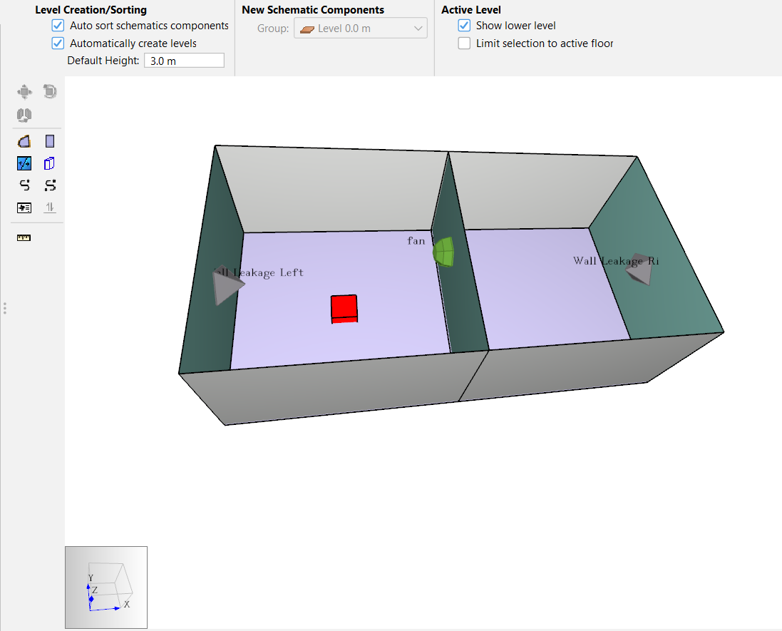
Open the modeling-doors-start.vnts model from the zip in Before Starting. It should resemble Figure 1.
Use the Analysis › Simulation Parameters action to open the Simulation Parameters dialog.
Select Steady for Airflow Simulation Method and Steady for Contaminant Simulation Method.
Select OK.
Save the file as performance-curve-demo.vnts

Define the New Flow Elements

To model the fan

Use the Model › Edit Flow Elements action to open the Edit Flow Elements dialog.
Click New to open the New Flow Element dialog.
Enter the name Fan 1 and select the Performance Curve model.
Click OK to create the new Flow Element.
In the dialog for the Fan 1 element, click the Edit… button next to Fan Performance Data.
In the Edit Performance Curve Data dialog, Confirm the [default] values match Table 1.

Table 1. Performance Curve Points for "Fan 1"

Flow (kg/s)	Pressure Rise (Pa)
0.0	150
2.0	125
3.0	110
4.0	60

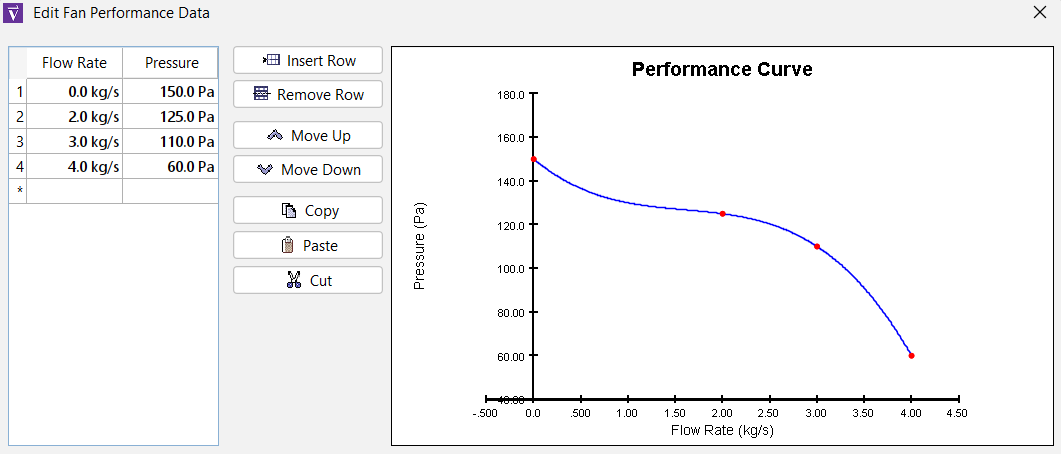
Click OK to close the performance curve data editor.
Enter 0.5 in the Flow Exponent field, a Cut-off Ratio of 0.5 (50%), and 0.1 m² in the Equivalent Orifice Area field.
Click Apply to save the changes. The dialog should match Figure 3.

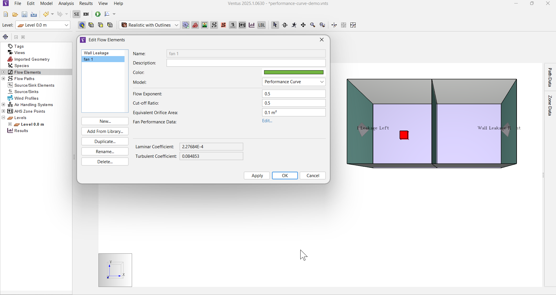
Figure 3. Creating the Flow Elements in the model

Click OK to apply the changes.

The Flow Element is now ready for use in Flow Paths.

Create the Flow Paths

We will create one fan object with a performance curve Flow Path between the Zones.

Click the icon to switch to the Top View.
Double-click the icon to select the Two Point Flow Path tool in pinned mode.
In the Tool Properties ribbon, select the Fan 1 Flow Element in the Element field.
Drag to draw a line across the wall between the two Zones to create a Flow Path modeling the fan.
Switch to the Perspective View. The model should look like Figure 4.

Completed Model — Figure 4. The completed model.

The Flow Paths are now created.

Define the Multiplier Schedule

In the workspace or object panel, select the Flow Path you just created
Rename the Flow Path fan 1.
In the Multiplier dropdown of the Properties Panel, select Schedule.
Click the hyperlink t(0) =… to open the Edit Multiplier dialog.
Enter 0.25 in the initial value field and select OK.

The Multiplier Schedule imposes a speed ratio onto the fan 1 Flow Path. The fan is OFF at 25 % speed ratio. Because this speed ratio (0.25) is below the Cut-off Ratio value (0.50), the Flow Path should switch from modeling performance curve data to modeling an Orifice Area.

Run the Simulation

We are now ready to run the simulation.

Click the Run icon . The simulation should take only a few seconds.
When the simulation is complete, click OK in the Run Simulation dialog.

The simulation should complete in a matter of seconds, and you should see the 3D Flow Path visualizations update in real time, showing the flow vectors at each Flow Path.

Results for below cut-off operation

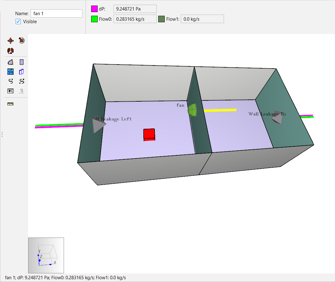
Figure 5. Results below cut-off (the fan 1 pressure drop vector is hidden inside the Flow Path graphic)

The solution in Figure 5 will result from any value of fan speed entered into the fan 1 schedule that is less than or equal to cut-off ratio.

As expected the fan 1 flow path mimics an Orifice Area Powerlaw flow model in Figure 5. The flow and pressure vectors (Flow0 and dP) are in the same direction. Flow from Supply01 moves air from Zone00 → Zone01; the pressure drop is positive from Zone00 to Zone01.

Next, let’s examine when the fan speed ratio is adjusted above the Cut-off Ratio.

Fan Flow Path above Cut-off

In this section, we demonstrate above cut-off behavior in a few steps:

Schedule a fan speed ratio above the Flow Element defined Cut-off Ratio.
Run the simulation and inspect the results.
Edit the Schedule and set up the model with a full-speed fan ratio.
Re-run the simulation and inspect the results.
Consider fan stall conditions.
Examine the fan performance at a different pressure requirement by modifying the AHS Supply setting.

Change the Multiplier Schedule

Select path fan 1 and in the Multiplier dropdown, select Schedule.
Click the hyperlink t(0) =… to open the Edit Multiplier dialog.
Enter 0.75 in the initial value field and select OK.

The Multiplier Schedule imposes a speed ratio onto the fan 1 Flow Path. The fan is ON at 75 % speed ratio. Because this speed ratio is above the Cut-off Ratio value, 50%, the fan model should use performance curve data to force airflow against the direction of pressure drop.

Re-run the Model

Click the Run icon .
When the simulation is complete, click OK in the Run Simulation dialog.

Results

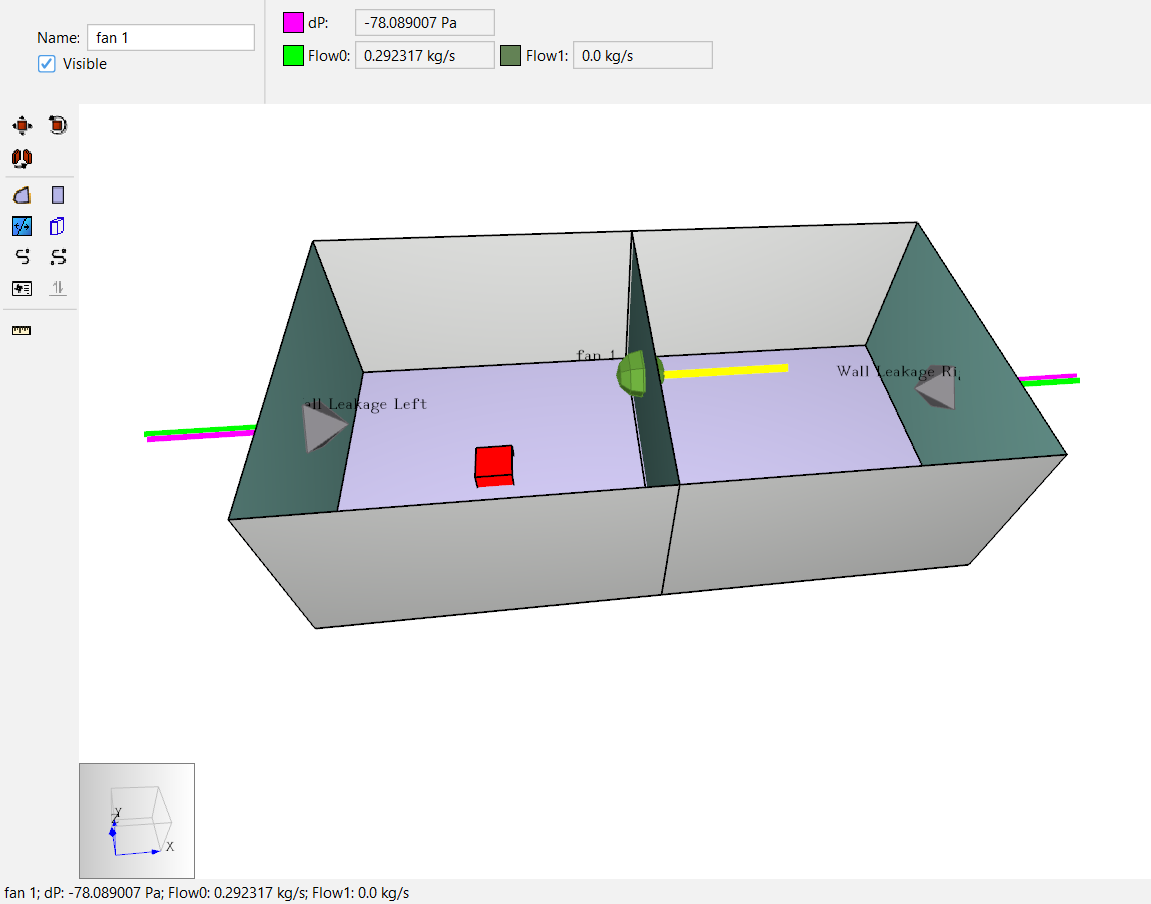
The solution in Figure 6 will result from 75% speed ratio only.

As expected, the fan 1 flow is defined by the performance curve data. In the workspace, the 3D flow and pressure drop vectors (Flow0 and dP) are in opposite directions. Forced flow from the fan 1 Performance Curve Data determines the flow and pressure between Zone00 and Zone01 as a function of the system requirements (computed in ContamX).

At 75% speed, the operating point is (0.2923 kg/s, -78.089 Pa).

Next, model the fan at full speed.

Change the Multiplier Schedule

Select path fan 1 and in the Multiplier dropdown, select Schedule.
Click the hyperlink t(0) =… to open the Edit Multiplier dialog.
Enter 1.0 in the initial value field and select OK.

The Multiplier Schedule imposes a speed ratio onto the fan 1 Flow Path. The fan is ON at 100 % speed ratio.

Re-run the Model

Click the Run icon .
When the simulation is complete, click OK in the Run Simulation dialog.

Results

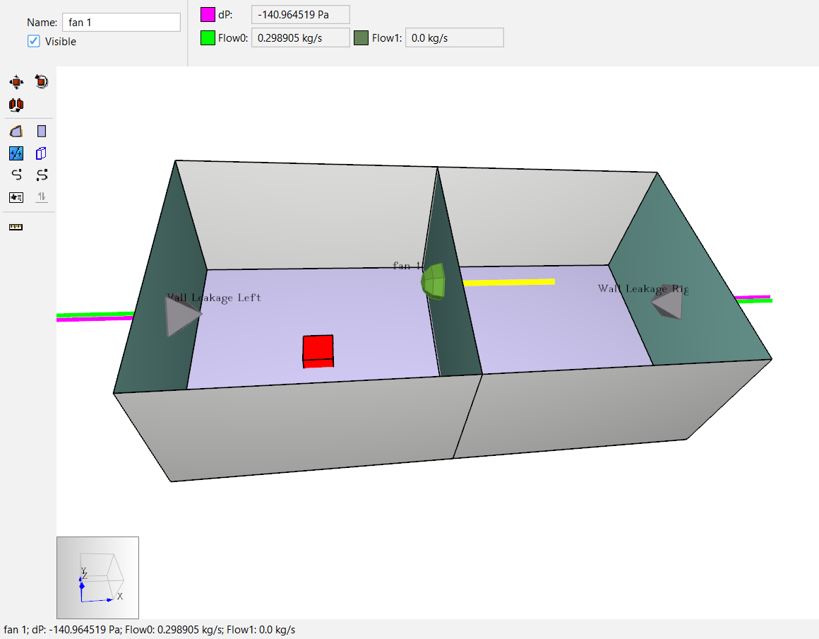
As in Figure 7, at 100% speed, the operating point is (0.2989 kg/s, -140.96 Pa). The flow rate has gone up only slightly and the pressure differential has significantly increased.

Consider stall

After running any above cut-off simulation with the Performance Curve Flow Element, check whether the fan 1 operating point is near the Y-Axis. Near the Y-Axis the fan may stall in the real world. Ventus results calculations do not account for stall.

Next, examine an operating point further from the Y axis.

Examine a different pressure requirement

To examine the fan performance across a lower pressure rise, we can eliminate the flow from Supply01. This will reduce the pressure requirement of the system (the building).

Change the AHS Supply Point

Select object Supply01 and in the Multiplier dropdown, select Constant.
Enter 0 in the value field.

The fan model should ONLY use performance curve data to force airflow against the direction of pressure drop (dP). Now, the pressure rise (-dP) of the fan will be smaller because it does not have to push against the AHS Supply.

Re-run the Model

Click the Run icon .
When the simulation is complete, click OK in the Run Simulation dialog.

Results

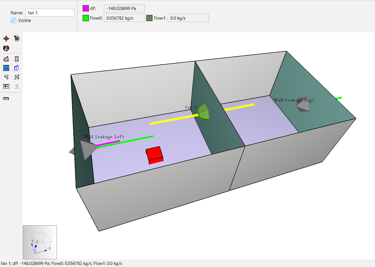
As in Figure 8, at 100% speed, with no AHS Supply flow, the operating point is (0.0568 kg/s, -148 Pa).

Change the Multiplier Schedule

Select path fan 1 and in the Multiplier dropdown, select Schedule.
Click the hyperlink t(0) =… to open the Edit Multiplier dialog.
Enter 0.75 in the initial value field and select OK.

The Multiplier Schedule imposes a speed ratio onto the fan 1 Flow Path. The fan is ON at 75 % speed ratio.

Re-run the Model

Click the Run icon .
When the simulation is complete, click OK in the Run Simulation dialog.

Results

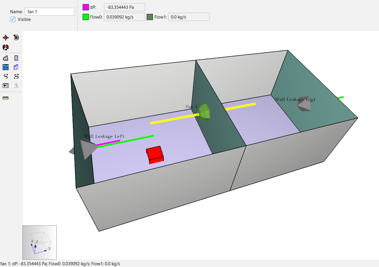
As in Figure 9, at 75% speed, the operating point is (0.03909 kg/s, -83.35 Pa).

Compare Results

In this section, we compare results data for the results in Fan Flow Path below Cut-off and Fan Flow Path above Cut-off with simple post-processing:

Tabulate the complete results data.
Use a plot to create the beginning of a performance curve for each fan speed.
Check the above cut-off fan behavior against the user-defined Performance Curve.

Results Table

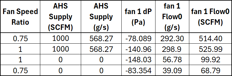
The complete data for the demo is in Table 2.

Table 2. Compiled results table

Multiplier	Above Cut-off	Flow (g/s)	Pressure Drop (Pa)
0.25	No	283	9.25
0.75	Yes	292	-78.1
1.0	Yes	299	-141
1.0	Yes	56.8	-148
0.75	Yes	39.1	-83.4

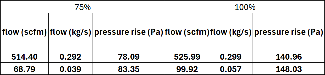
Only the Above Cut-off results are useful to fan performance analysis. When those relevant results are reorganized and converted into airflow units of SCFM, the data looks like Figure 10. When the data is sorted to represent each fan speed setting and pressure drop is converted to pressure rise, the data appears as in Figure 11.

Fan Table 1 — Figure 10. AHS settings and Fan data table formatted in order of how-to steps

Fan Table 2 — Figure 11. Fan data table formatted with separate fan speed results

Results plot

These points can be plotted to establish the beginning of a performance curve for each fan speed.

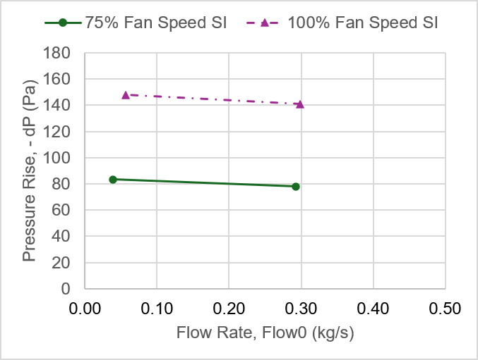
Values for 100% speed can be compared directly with the performance curve plot in Ventus. Visually compare Figure 12 to Figure 13.

The completed VNTS model and the Excel workbook with tabulated data and the plot in Figure 12 can be accessed here: performance-curve-completed.zip

Conclusion

You should now be familiar with how to model fan devices with user-defined performance curve data. You should also understand the impact of Cut-off Ratio and the Multiplier Schedule / fan speed ratio input.

Use this technique in your own models to increase the scope of your simulations.

To download the most recent version of Ventus, please visit the Ventus download page. Please contact support@thunderheadeng.com with any questions or feedback regarding our products or documentation.

Modeling Fans: Performance Curves

To model the fan

Related Tutorials