Velocity Patch in FDS

Reading Time: 4 minutes

Created with software version: 2020.1

1. Introduction

As part of exploring options to model jet fans (see our Jet Fan Tutorial), we looked at using a Velocity Patch. The FDS User Guide discusses the concept of a velocity patch in the context of air entrainment by the spray from a sprinkler nozzle. The idea is that the spray droplets accelerate the gas through which they move and a velocity patch gives a way to specify the gas velocity. We sought to apply a velocity patch to a model of a jet fan.

2. Velocity Patch Background

As described in the FDS User Manual (Section 15.3.3), "The details of the sprinkler head geometry and spray atomization are practically impossible to resolve in a fire calculation. As a result, the local gas phase entrainment by the sprinkler is difficult to predict. As an alternative, it is possible to specify the local gas velocity in the vicinity of the sprinkler nozzle."

A velocity patch consists of:

A bounding volume
A cartesian point (XYZ)
Polynomial coefficients that define the velocity using a second order Taylor expansion about the cartesian point XYZ. The polynomial is specified by the coefficients:
- P0 - the value of the velocity component (k)
- PX(1:3) - the first derivatives at cartesian point XYZ
- PXX(1:3,1:3) - the second derivatives at cartesian point XYZ

Velocity Patch Equation

\[\mu_k \left( r \right) = \underbrace{\left( \mu_k \right)_0}_{P0} + \underbrace{r_i \left( \frac{\delta \mu_k}{\delta x_i} \right)_0}_{PX(1:3)} + \frac{r_ir_j}{2} \underbrace{\left( \frac{\delta^2 \mu_k}{\delta x_i \delta x_j} \right)_0}_{PXX(1:3,1:3)}\]

If we want a constant velocity, we only specify P0. The first line of the FDS input in Figure 1 defines the velocity component (in this case the X direction) and the constant value, P0. The second line defines a timer that activates the patch. The third line defines the geometry of the patch and links the patch to the previous data. By default the point XYZ is the center of XB, but as will be shown below, you can add a point definition to this line to shift the center of the expansion.

fds scrn velpatch constant — Figure 1. Velcoity Patch, Constant Velocity

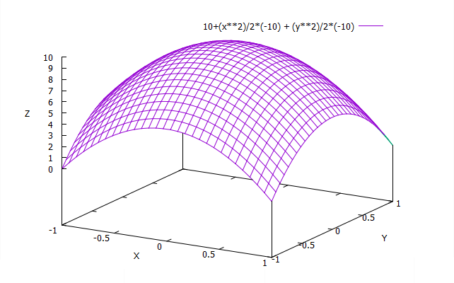
For a parabolic velocity in the X direction that varies in the Y-Z plane, the Taylor expansion simplifies to:

Simplified Taylor Expansion

\[u \left( r \right) = P_0 + \frac{y^2}{2} \left(P_{22} \right) + \frac{z^2}{2} \left( P_{33} \right)\]

The plot shows the velocity for a patch that extends from Y=-1 to Y=1 and Z=-1 to Z=1, with latex:[TCP_{mpp}] and \(P_{22}=P_{33}=-10\).

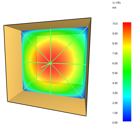
gnuplot velpatch parabolic — Figure 2. A parabolic velocity patch with the centerline velocity of 10 and 0 at the corners of the patch.

This was tested in PyroSim using the following FDS input data:

fds scrn velpatch parabolic input — Figure 3. Parabolic Patch FDS Input Data

which resulted in the contours shown in Figure 4 that match the expected results.

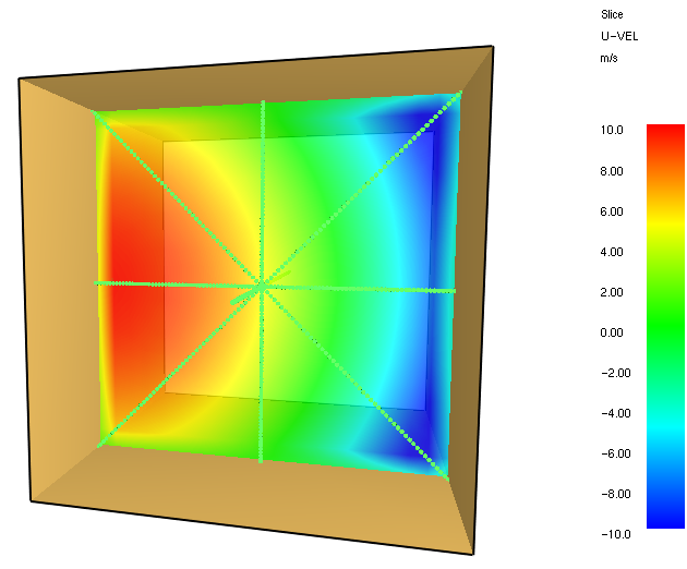
results scrn velpatch parabolic results — Figure 4. Test case for a parabolic velocity distribution with 10 at the centerline and 0 at the corners of the velocity patch.

To demonstrate shifting the XYZ point for the Taylor expansion from the center to the edge at Y=1, we add XYZ data to the velocity patch device:

fds scrn velpatch shifted parabolic input — Figure 5. Parabolic FDS Patch Shifted Input

This results in the countours shown in Figure 6:

results scrn velpatch shifted parabolic — Figure 6. Test case for a parabolic velocity with the point XYZ located at 1,1,0.

3. Applications

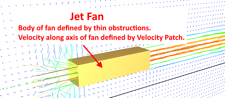
The velocity patch makes it possible to define the gas velocity components within a given volume. For a sprinkler, this allows the user to specify the gas velocity caused by the spray droplets. We tested a model of a jet fan, shown in Figure 7 by making a shroud of thin obstructions and specifying the velocity of the gas along the axis of the fan using a velocity patch.

In the end, using a velocity patch to model a jet fan is probably not the best approach, but it does demonstrate one uncommon feature of FDS.

pyro scrn velpatch jet model — Figure 7. A jet fan modeled using thin obstructions for the fan body and a velocity patch to define the gas velocity in the fan in the direction of the fan axis.

To download the most recent version of PyroSim, please visit the the PyroSim Support page and click the link for the current release. If you have any questions, please contact support@thunderheadeng.com.

Related Tutorials

Modeling Jet Fans Reading Time: 28 minutes

Tutorial demonstrating how to model jet fans in Pyrosim.

- jetfan calcs experiment flow hvac mesh output

(Legacy) PyroSim Fundamentals Reading Time: 3 minutes

(Legacy) Tutorial to experience the fundamental features of PyroSim

- presentation cad combustion control device flow geometry hvac import material mesh output pyrolysis radiation surf

HVAC Pressure Drop Verification Reading Time: 2 minutes

Tutorial demonstrating how to verify HVAC Pressure Drop in Pyrosim.

- calcs devices flow hvac output

Critical Velocity in Tunnel Fires Reading Time: 6 minutes

Tutorial demonstrating how to model critical velocity in Pyrosim using the example of a tunnel fire.

- tunnel calcs experiment flow output

Radiation and Convection on Surfaces Reading Time: 5 minutes

Tutorial demonstrating how to model Radiation and Convection on Surfaces in Pyrosim.

- device experiment heat transfer material output radiation surf

Using PyroSim/FDS to Maximize Solar Panel Convective Cooling Reading Time: 12 minutes

Tutorial demonstrating how to use PyroSim/FDS to Maximize Solar Panel Convective Cooling.

- cad experiment flow heat transfer material mesh output radiation

Smoke Visibility and Obscuration Reading Time: 13 minutes

Tutorial demonstrating how to model Smoke Visibility and Obscuration in Pyrosim.

- vnv calcs device experiment

Basic First Model Reading Time: 13 minutes

To demonstrate basic Ventus (and CONTAM) capability, we will model a simple six-story building for winter and summer conditions.

- flow geometry import output contam