To follow along with this tutorial, download the relevant files here.
Introduction
Solar panels are most efficient if they operate at lower temperatures. When designing a solar panel installation the question might arise, "What is the best solar panel spacing to maximize solar panel convective cooling?" This post uses PyroSim and FDS to evaluate some different solar panel mounting options to maximize solar panel convective cooling in a real world example of a solar panel installation.
Standard tests are used to measure solar panel performance parameters.
The IEC 61215 test procedure measures the Nominal Operating Cell Temperature (NOCT).
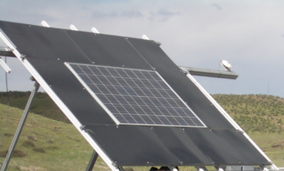
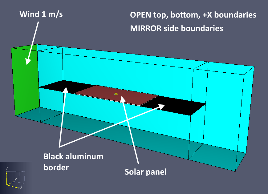
This is the temperature reached by a solar panel when exposed to a solar irradiance of 800 W/m2, air temperature of 20 ºC, wind velocity of 1 m/s, mounted at 45º with the back side open, and with open circuits, shown in Figure 1.
The panel is surrounded by a 0.6 m black aluminum plate border.
The Temperature Coefficient of Power at Maximum Power Point voltage (\(TCP_{mpp}\)) is the change in power with change in temperature.
From the SolarWorld SW 340 data sheet for the panels used in our real world example, NOCT=46 ºC and \(TCP_{mpp}\) = -0.43%/ºC.
So an increase in temperature of 20 ºC will result in an 8.6% drop in power.
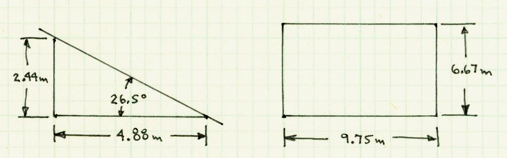
The roof that these panels will be installed on will have a 26.5º slope, a length of 9.75 m (32 feet), and a rafter span including overhang of 6.67 m (21.88 feet), shown in Figure 2.
Each panel is 1.993 m (78.46 inches) long and 0.961 m (37.8 inches) wide.
The roof slope is somewhat less than the optimum value of 33.5º for latitude 40º.
Panels are supported on rails that leave a gap of about 16.5 cm (6.5 inches) between the bottom of the panel and the roof.
This gap allows air to flow under the panel and cool the panel.
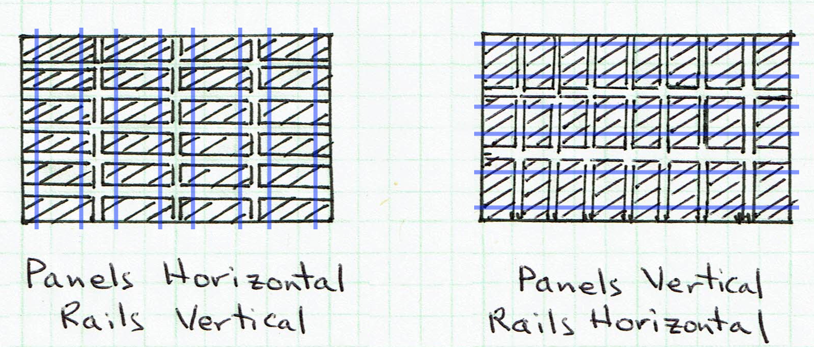
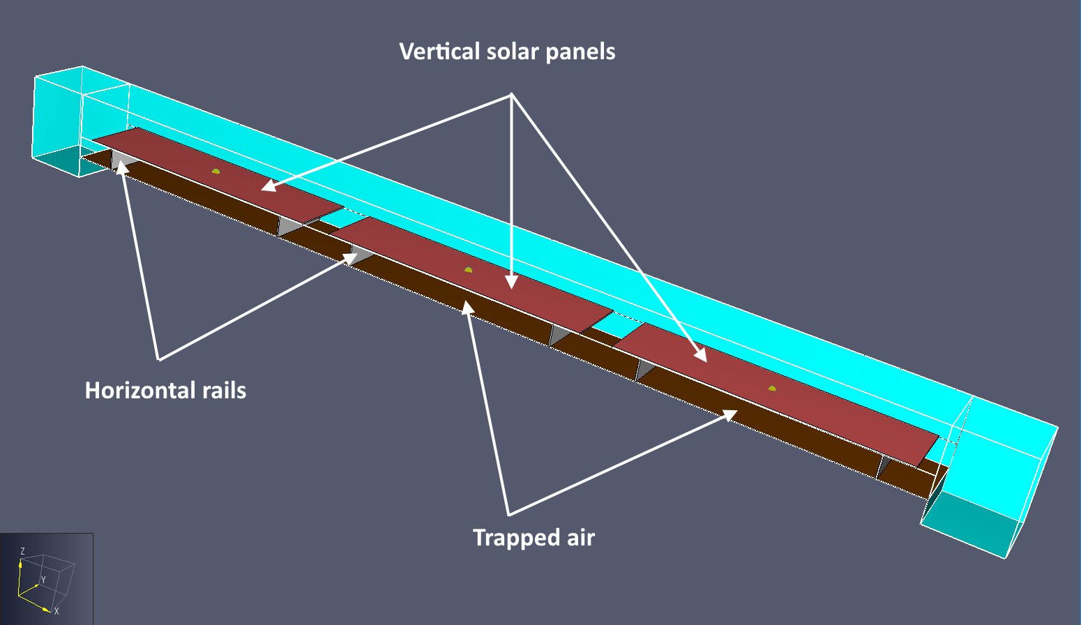
The warranty requires that the rails cross the long side of the panels, giving two options for orientation as shown in Figure 3.
When the panels are horizontal, the vertical support rails provide a clear path for convective air flow.
When the panels are vertical, the horizontal support rails block the convective flow under the panels.
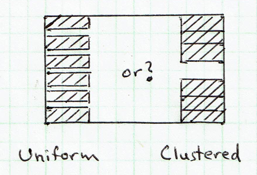
In addition to the orientation, we can use different arrangements of the space between panels, demonstrated in Figure 4. Should the spacing be uniform, or it is better to cluster panels together with a large gap between the clusters?
Modeling Details
The same modeling approach was used for all simulations. In general, the models are standard, but there are a few details that deserve discussion:
- Specifying the solar irradiance using the EXTERNAL_FLUX parameter on the surface.
- Using a layered material and EXPOSED backing to incorporate heat conduction from the front to back surface of the panels.
- Rotating the gravity vector relative to the model axis.
- Using MIRROR (symmetry) boundary conditions on the sides of the model.
These details are discussed below.
Solar Irradiance
While it would be possible to directly model the sun using a hot obstruction, the easiest way to specify the solar irradiance is to define an EXTERNAL_FLUX on the solar panel.
This option is not currently supported in the PyroSim interface, so when defining the surface exposed to the sun, on the Edit Surfaces dialog click the Advanced tab and type EXTERNAL_FLUX for the parameter name and the value of irradiance (kW/m2).
For these calculations, the value was 0.8 for the IEC 61215 simulations and 1.0 for the solar panel calculations.
Heat Conduction from Front to Back Surface
Heat conduction in FDS is one-dimensional and, except in the case of the EXPOSED option, each face of an obstruction is calculated independently by assuming the back side of each face is either insulated or open to ambient conditions. If the obstruction is less than or equal to one mesh cell thick, and if there is a non-zero volume of computational domain on the other side of the wall, the EXPOSED option will couple the temperature of the front side to the back side to enable heat conduction from front to back. The thickness and material used to perform the calculation are specified as part of the surface properties (the thickness used for heat conduction is independent of the geometry of the obstruction). In PyroSim, these values are specified on the Material Layers and Surface Props tabs of the Edit Surfaces dialog.
For the solar panels, no heat transfer or emissivity information was available.
The artificial material used had properties for aluminum, with a reduced heat capacity.
The panel was assumed to be 1 cm thick.
Using aluminum conductivity means that heat conduction through the thickness was large so the back panel face temperature was only slightly lower than the front temperature.
Assuming high conductivity is consistent with wanting to identify the effect of convection heat transfer from the back surface.
Since we are only interested in the steady state temperature of the panel, the heat capacity of the aluminum material was reduced by approximately a factor of 10.
This does not change the steady state solution, but does speed the transient calculation from the initial ambient conditions to the final steady state conditions.
An emissivity of 0.9 was assumed for the solar panel.
One case was run to determine an upper bound front temperature by assuming the back of the panel was insulated, so there was no heat removal from the back.
The thickness of the obstruction was less than one cell to satisfy that FDS requirement.
Rotated Gravity Vector
FDS uses a rectilinear grid system.
A sloped surface not aligned to the grid is represented by a stair-stepped mesh.
For these simulations, the stair-stepped mesh can be avoided by building the model aligned to the rectilinear grid and rotating the gravity vector to represent the slope, 45º for the IEC 61215 model and 26.5º for the real world example.
This is done on the Environment tab of the Simulation Parameters dialog.
For the 26.5º slope, the gravity vector has an X component of -4.376 m/s2 and a Z component of -8.774 m/s2.
MIRROR Symmetry on Side Boundaries
To speed the solution, the model represents a 0.5 m slice through the panels.
The boundaries on the side of the model could either be OPEN, MIRROR, or PERIODIC.
Because just a section of a panel was modeled, the MIRROR option was used for the side boundaries.
This is a symmetric boundary condition with a no-flux, free-slip boundary.
IEC 61215 Simulations
The IEC 61215 model is shown in Figure 5.
Solar irradiance of 800 W/m2 was specified for both the black aluminum border and the solar panel.
The gravity vector was rotated 45º to represent the tilted panel.
Boundary conditions were MIRROR on the sides, a specified wind velocity of 1 m/s on the -X boundary, and OPEN on all other boundaries.
The emissivity of the panel was assumed to be 0.9 and of the black border 1.0.
If the emmissivity is less, this would reduce the temperature of the panel.
The mesh size for all models was 2.5 cm.
Results
Figure 6 shows the temperatures of the top and bottom of the solar panel, measured at the center of the panel.
The top and bottom temperatures are essentially identical, so the curves lie on top of each other.
The steady state value is 55.1 ºC, compared to the data specification sheet value of 46 ºC.
The emissivity of the panel could be reduced to calibrate the calculation to the match the data sheet.
No calibration was performed since changes in temperature caused by different panel configurations should not be sensitive to small changes in emissivity.
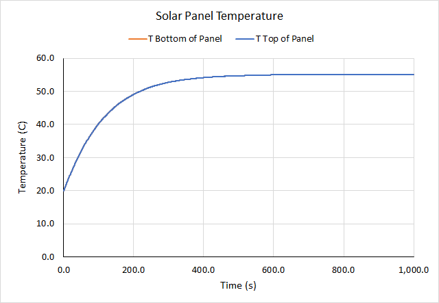
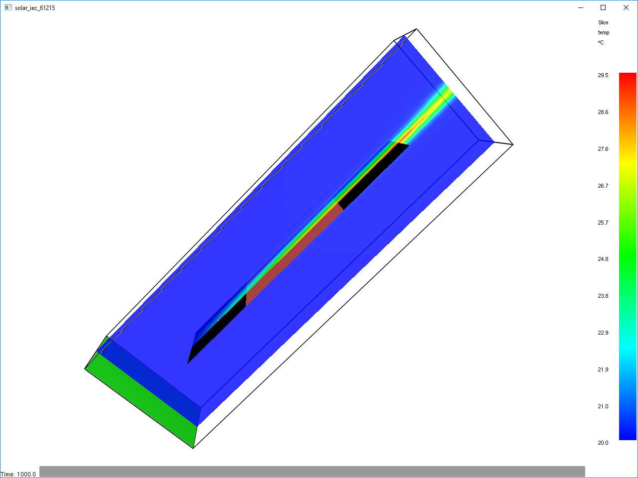
Figure 7 shows the air temperature contours on a slice through the center of the panel.
The IEC 61215 panel had a temperature of 62.7 ºC when the solar irradiance was increased to 1000 W/m2.
Solar Panel Layout Simulations
Now we look at the temperatures of panels installed on the roof.
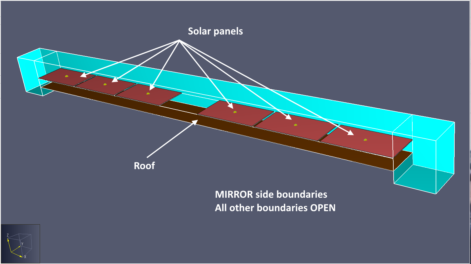
Figure 8 shows the model for the roof-mounted panels with a large 75 cm gap between two clustered arrays.
The panels in this model are arranged in the "panels horizontal, rails vertical" orientation shown in Figure 3.
The model represents a 0.5 m slice through the array.
As the panels are heated by solar irradiance, air flows between the solar panels and the roof. The roof is assumed to be insulated, so it will be warmed by radiation from the solar panels and convection as the flowing air is heated.
The second model is similar to the large central gap model, but all the panels are arranged in one tightly packed cluster with a uniform gap of 4 cm between them.
The third model, shown in Figure 9, represents a slice of the "panels vertical, rails horizontal" installation of Figure 3. Because the rails are horizontal and we assume MIRROR (symmetry) conditions for the side boundaries, air is trapped under the panels.
The final case assumed that the solar panels were insulated, so were not cooled by air flow under the panels. This used the close-packed model configuration, modified to insulate the panels. The purpose of this case is to examine the maximum temperature that the panels could reach.
In all cases, the emissivity of the panels and roof was assumed to be 0.9, consistent with the IEC 61215 simulations.
As noted, this emissivity was not calibrated to give the NCOT temperature of the data sheet.
If calibrated, the temperature would be lower, but changes in temperature due to different panel configurations should not be sensitive to small changes in emissivity.
The mesh size for all models was 3.3 cm.
Results
Figure 10 shows air temperature contours for the large central gap model after the panels had reached steady state temperature. Note that the flow is not steady state, but is turbulent over the panels. Figure 11 shows the flow vectors near the central gap. At this instant of time, some fresh air is being drawn into the central gap that cools the flow under the upper grouping of panels.
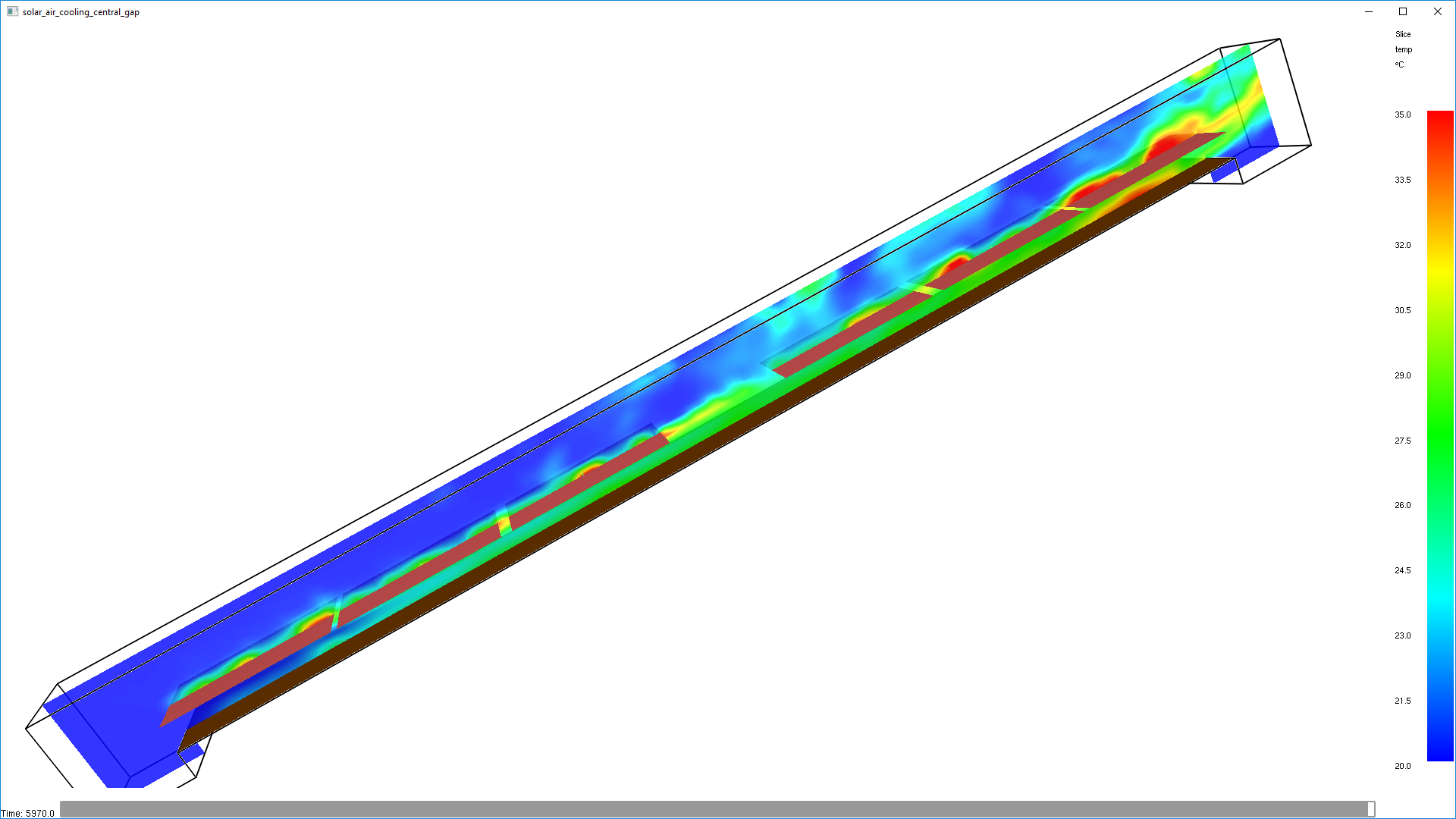
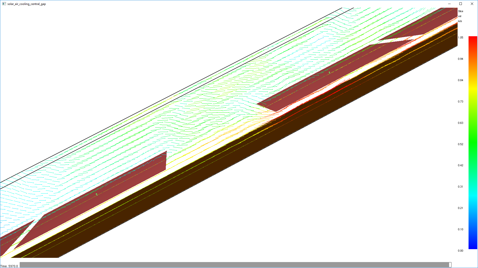
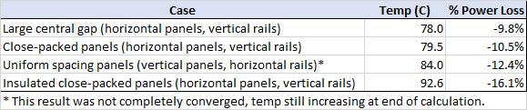
Figure 12 summarizes the results of this study. For all cases with horizontal panels, the temperatures are given for the 4th panel. This is the panel just above the large central gap. For the vertical panels, the temperature is for the 2nd panel, the central panel for that configuration.
Mesh Convergence Study
A mesh convergence study was performed in which the cell size was reduced by a factor of 2 in all directions, giving 8 times more cells.
The calculated temperature for the refined mesh was 0.3 ºC higher than the original mesh, so the results are considered converged with respect to mesh size of 3.3 cm.
Summary
The results for the IEC 61215 test gave an NCOT of 55.1 ºC, which is higher than the data sheet value of 46 ºC.
The emissivity of the panel could have been reduced to calibrate the calculation to the match the data sheet, but emissivity was not calibrated since changes in temperature caused by different panel configurations should not be sensitive to small changes in emissivity.
For consistency, the calculated NCOT of 55.1 ºC was used to calculate power loss for the roof mounted panels.
When panels are mounted on a roof, the flow between the panels and the roof can help cool the panels.
Relative to IEC 61215 panels which are mounted at 45º with the back side open, the roof mounted panels run about 25 ºC hotter.
This corresponds to a power loss of about 10%.
There was not a large difference due to close-packed or central gap mounting of the horizontal panels.
Vertical panels with horizontal rails show an increased temperature and additional power loss that would probably be at least 5% if the calculation were continued to convergence, data shown in Figure 12.
If there is no bottom surface cooling of the panels, the power loss was about 16% relative to the IEC 61215 calculation.
As shown by these calculations, the real world panels are expected to run hotter than the NCOT temperature. Unfortunately, the reasons the panels will run hotter are primarily due to uncontrollable parameters:
- The expected peak solar irradiance will be larger than in the NCOT test.
- Because of the roof installation, the back of the panels is not open to free air flow.
- The panels will be installed at a slope of
26.5º, which is less than the45ºslope in the NCOT test. This reduces convective flow.
These calculations did show that it was advantageous to mount the panels horizontally with vertical rails.
To download the most recent version of PyroSim, please visit the the PyroSim Support page and click the link for the current release. If you have any questions, please contact support@thunderheadeng.com.
Bibliography
Muller, Matthew. 2010. “Measuring and Modeling Nominal Operating Cell Temperature (NOCT).” Performance Modeling Workshop, September. https://www.nrel.gov/docs/fy10osti/49505.pdf.
Related Tutorials
(Legacy) Tutorial to experience the fundamental features of PyroSim
Tutorial demonstrating how to model Radiation and Convection on Surfaces in Pyrosim.
Tutorial demonstrating how to model jet fans in Pyrosim.
Tutorial demonstrating how to create and FDS Velocity Patch in Pyrosim.
Tutorial demonstrating how to model Heat Conduction in Pyrosim.
Tutorial demonstrating how to model critical velocity in Pyrosim using the example of a tunnel fire.
Video tutorial demonstrating how to fix geometry problems related to DWG importation.
Tutorial Demonstrating how to model pressure leakage using Pyrosim