Smoke Visibility and Obscuration

1. Introduction

Smoke visibility and obscuration are critical outputs of a fire simulation. This post reviews how visibility is calculated in FDS, compares the calculation to experimental data, and discusses how smoke is visualized in the new PyroSim Results Viewer and in Smokeview. The comparison of VTT experimental images with predicted smoke visualization using PyroSim/FDS shows remarkably good correlation.

Visibility is the distance that an observer can identify an object relative to the background and obscuration is the amount that light intensity is reduced as it passes through smoke. The calculated visibility is often used as an occupant tenability requirement, while obscuration is used to display smoke visually. In this post we aim to describe and present some background on how visibility and obscuration are calculated in FDS, the core computation engine used in PyroSim. In particular, we want to ensure that the new PyroSim Results Viewer correctly reads FDS results and displays smoke correctly. 

Our primary references for FDS implementation and experimental validation are: The FDS User’s Guide (McGrattan et al. 2021), The SMV Verification Guide (Forney 2019), and the paper Experimental Validation of the FDS Simulations of Smoke and Toxic Gas Concentrations (Rinne, Hietaniemi, and Hostikka 2007). Background information on measurement of smoke extinction coefficient and visibility is given in the papers: Method for Measuring Smoke from Burning Materials (Gross, Loftus, and Robertson 1966), Specific Extinction Coefficient of Flame Generated Smoke (Mulholland and Croarkin 2000), Evaluation of the Planck mean absorption coefficients for radiation transport through smoke (Widmann 2003), and Studies on Human Behavior and Tenability in Fire Smoke (Jin 1997). A general discussion is given in the Smoke Production and Properties chapter of the SFPE Fire Protection Handbook (SFPE 2016).

2. Smoke Visibility and Obscuration

In a fire calculation using the simple chemistry approach, the smoke is tracked along with all other major products of combustion (McGrattan et al. 2021). This means that for every cell in the model, the smoke density is known. The light extinction coefficient, \(K\), is the key parameter used to calculate both visibility and light obscuration. The intensity \(I\) of monochromatic (single wavelength) light passing a distance \(L\) through smoke is attenuated as follows:

where \(I_{0}\) is the incident intensity.

The light extinction coefficient \(K\) can be calculated using the mass specific extinction coefficient \(K_{m}\) and the smoke density \(\rho_{s}\)

The default FDS value is \(K_{m}\) = 8700 m2/kg, with a suggested uncertainty of ±1100 m2/kg. This value is recommended for smoke generated by flaming fires by (Mulholland and Croarkin 2000), where they summarized the results of seven studies involving 29 fuels. For smoke generated by smouldering (pyrolysis), the value ranges from \(K_{m}\) = 4000 m2/kg to \(K_{m}\) = 5000 m2/kg, with the smaller value due to the low light absorption of this smoke. All experiments referenced in the Mulholland and Croarkin paper were performed using a wavelength \(\lambda\) = 366 nm, corresponding to red in the visible spectrum.

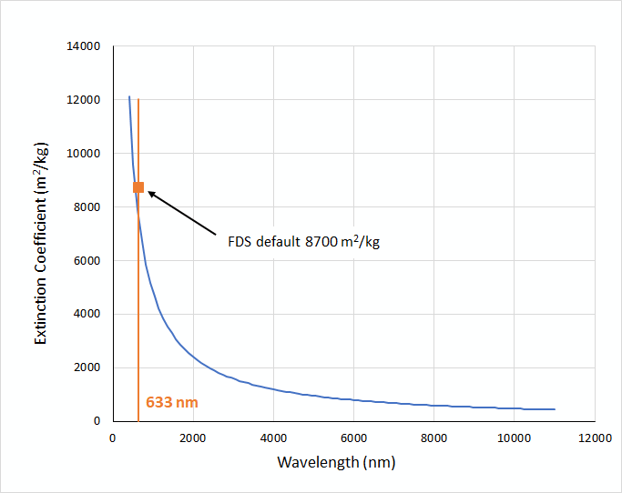
(Widmann 2003) analyzed data for flaming fires (stoichiometric and overventilated) and found the correlation between wavelength \(\lambda nm\) (nm) and \(K_{m}\) to be (equation 3):

This is plotted in Figure 1. The visible light spectrum extends from about 400 nm (violet) through 700 nm (red). Evaluating Wavelength - Mass Specific Extinction Correlation at a wavelength of 633 nm (the wavelength used to obtain the default \(K_{m}\) in FDS) gives an extinction coefficient of 7626 m2/kg, which is smaller than the default value used in FDS (8700 m2/kg), but near the recommended lower uncertainty limit. 

Once the light extinction coefficient K is known, the visibility is calculated using:

where (Jin 1997) recommends a range \(C\) = 2~4 for a reflecting sign and \(C\) = 5~10 for an illuminated sign. The default value used in FDS is \(C\) = 3. The experiments used to determine these values used signs in a smoke-filled chamber observed from outside through a glass window, so visibility was not affected by smoke irritation. The visibility measurement relied on the test subjects to determine the distance at which the object was no longer visible, not on a measurement of contrast.

We can see that there are several uncertainties in the calculation of obscuration and visibility. There are uncertainties in soot yield, uncertainties in extinction coefficient as a function of soot density, and uncertainties in calculating visibility as a function of extinction coefficient. The default values used in FDS should be considered reasonable for flaming fires and visibility of reflecting signs.

3. Verification Problem

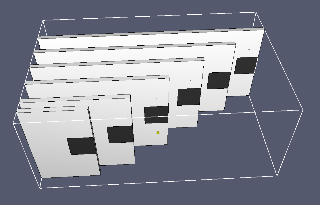
We will now verify the display of smoke in the Results Viewer integrated into PyroSim. The verification problem is based on the smoke_test problem presented in Chapter 3 of the Smokeview Verification Guide (Forney 2019). Figure 2 shows the model. White obstructions (gray scale 255) are positioned at distances of 0.5 m, 1.0 m, 2.0 m, 3.0 m, 4.0 m and 5.0 m depth. Black patches (gray scale 50) are positioned on the obstructions to evaluate contrast and visibility. The smoke density is uniformly initialized to a value of 7.922E-5 kg/m3. This gives a light extinction coefficient of 0.6889, corresponding to an intensity drop of 0.5 after passing through 1 m of smoke. 

The Weber contrast \(C\) has been discussed by (Mulholland and Croarkin 2000) and used experimentally by Cleary (2004).

The Weber contrast is calculated by:

where \(B\) is the brightness of the object and \(B_{0}\) is the brightness of the background.

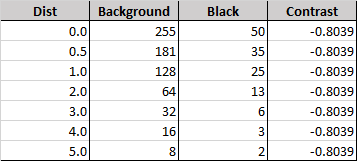
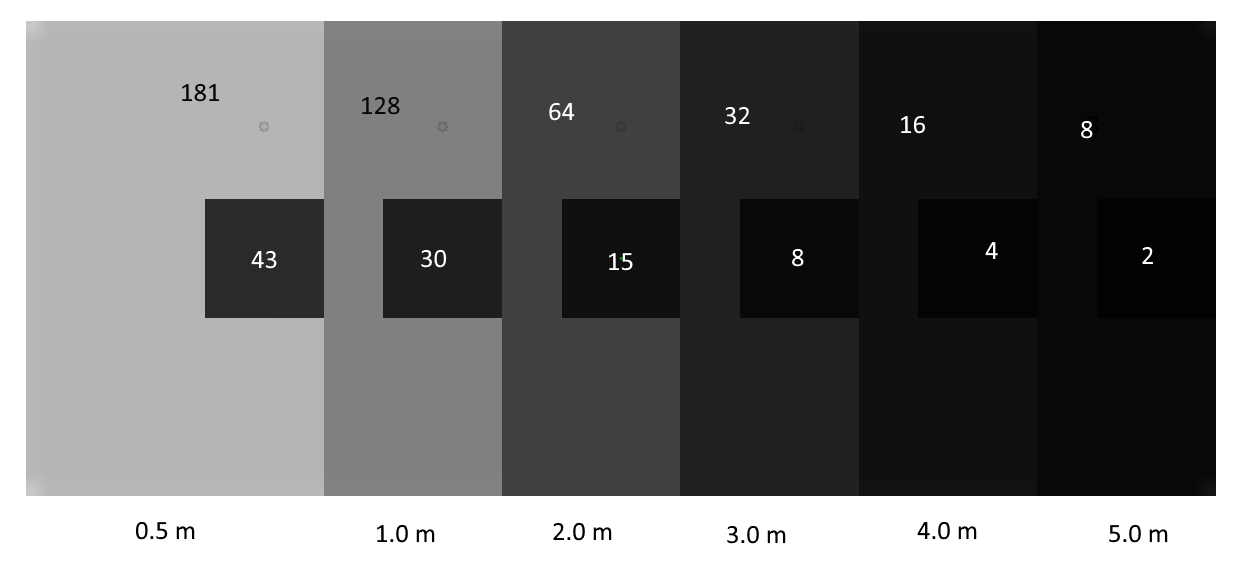
Mulholland notes that for a black object viewed against a white background, a value of \(C\) = -0.02 is often used as the contrast threshold defining visibility.  The expected light intensity of the white obstructions and the black patches are given in Figure 3, including the calculated Weber contrast. In this problem, both the background and the black patch are obscured equally by smoke, so that the intensity of both are reduced identically and the calculated Weber contrast is constant. As will be shown, the visibility is clearly reduced with increased obscuration, so it appears that the Weber contrast is not useful in calculating visibility in such a situation. An additional problem with the Weber contrast is that for a pure black object (gray scale 0), Weber Contrast Equation will give a constant value of -1. 

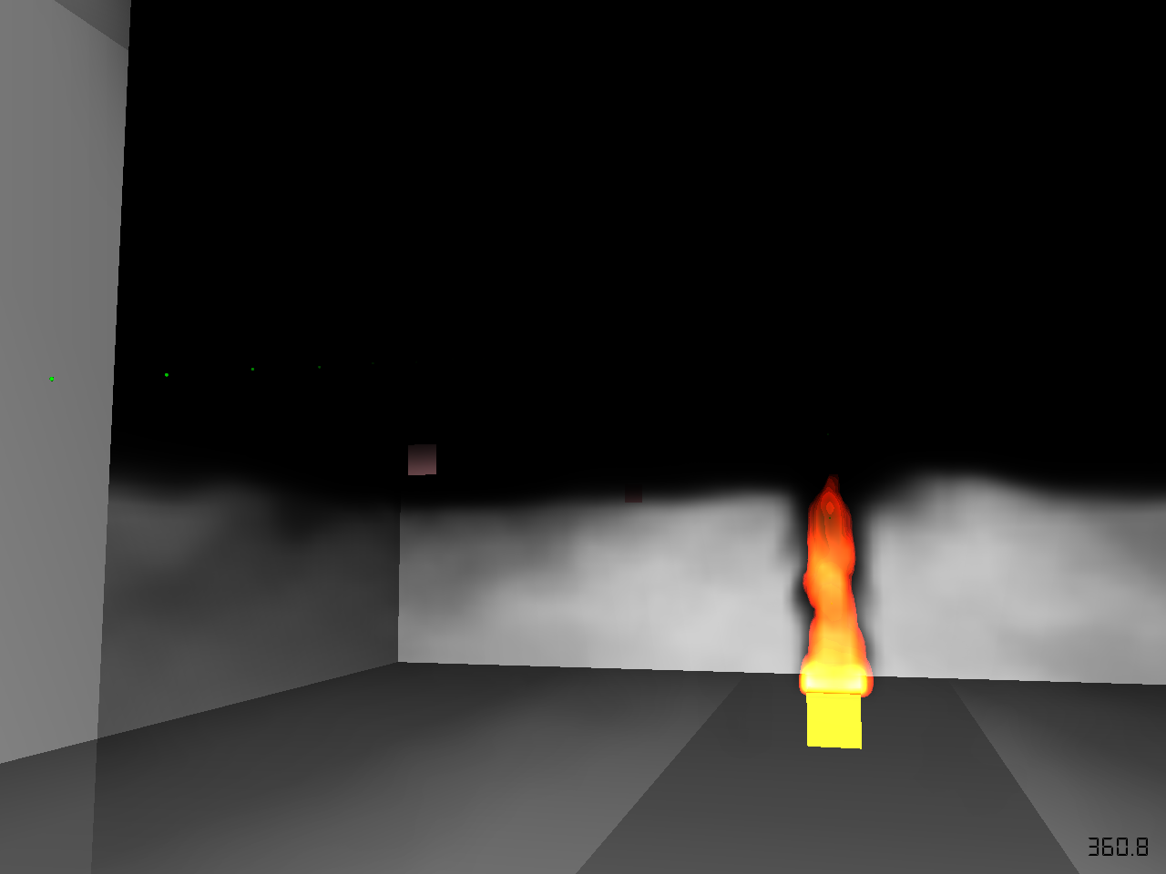
The FDS and PyroSim Results Viewer of the smoke are shown in Figure 4. The theoretical and displayed values are identical. Based on the extinction coefficient, the visibility is 4.35 m. A careful examination of Figure 4 shows that we can just discern the black patch at a distance of 4.0 m, but cannot identify the patch at 5.0 m, so the visibility calculation matches the display. However, this also demonstrates that the Weber contrast cannot be used to determine visibility in such a case. 

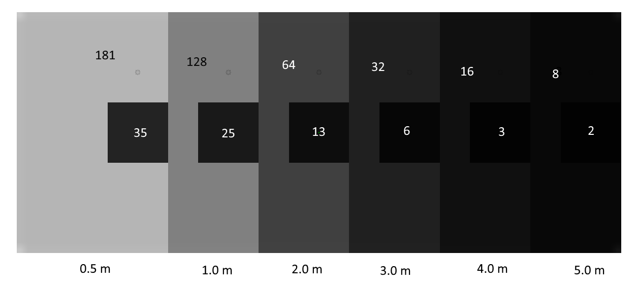
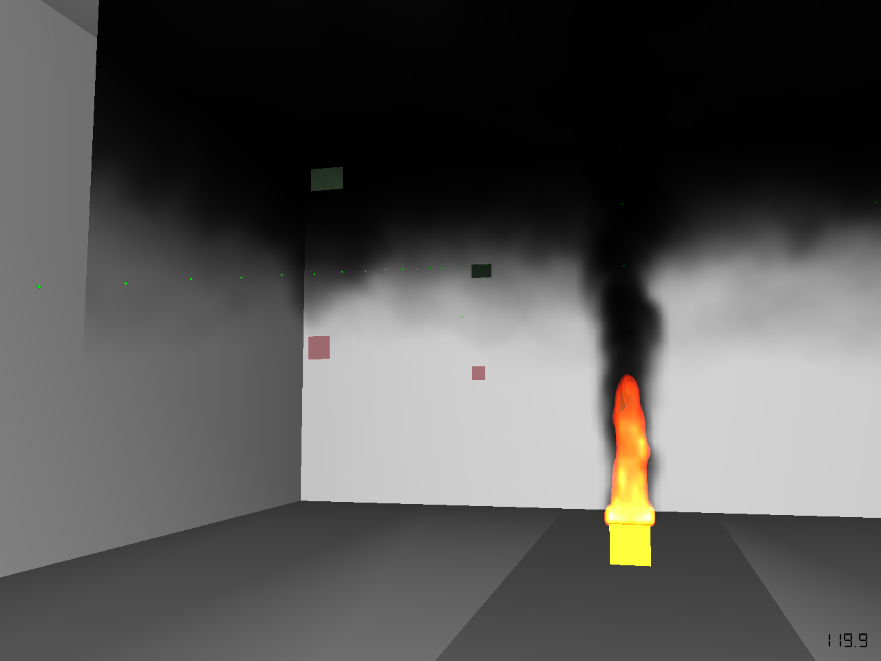
It should be noted that in Figure 4, the ambient light was set to zero and camera light was positioned at infinity. Figure 5 shows the results using the default ambient light (0.2) and the default light position at the camera. The ambient light value does not change the intensity of the white obstructions, but the dark gray patches appear somewhat lighter.

4. VTT Experimental Validation of Visibility

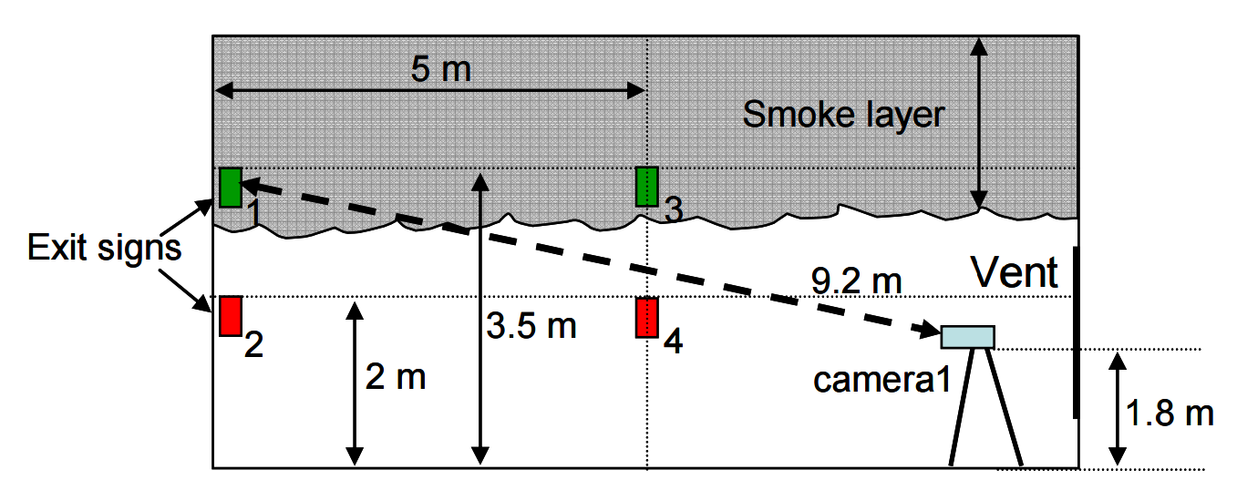
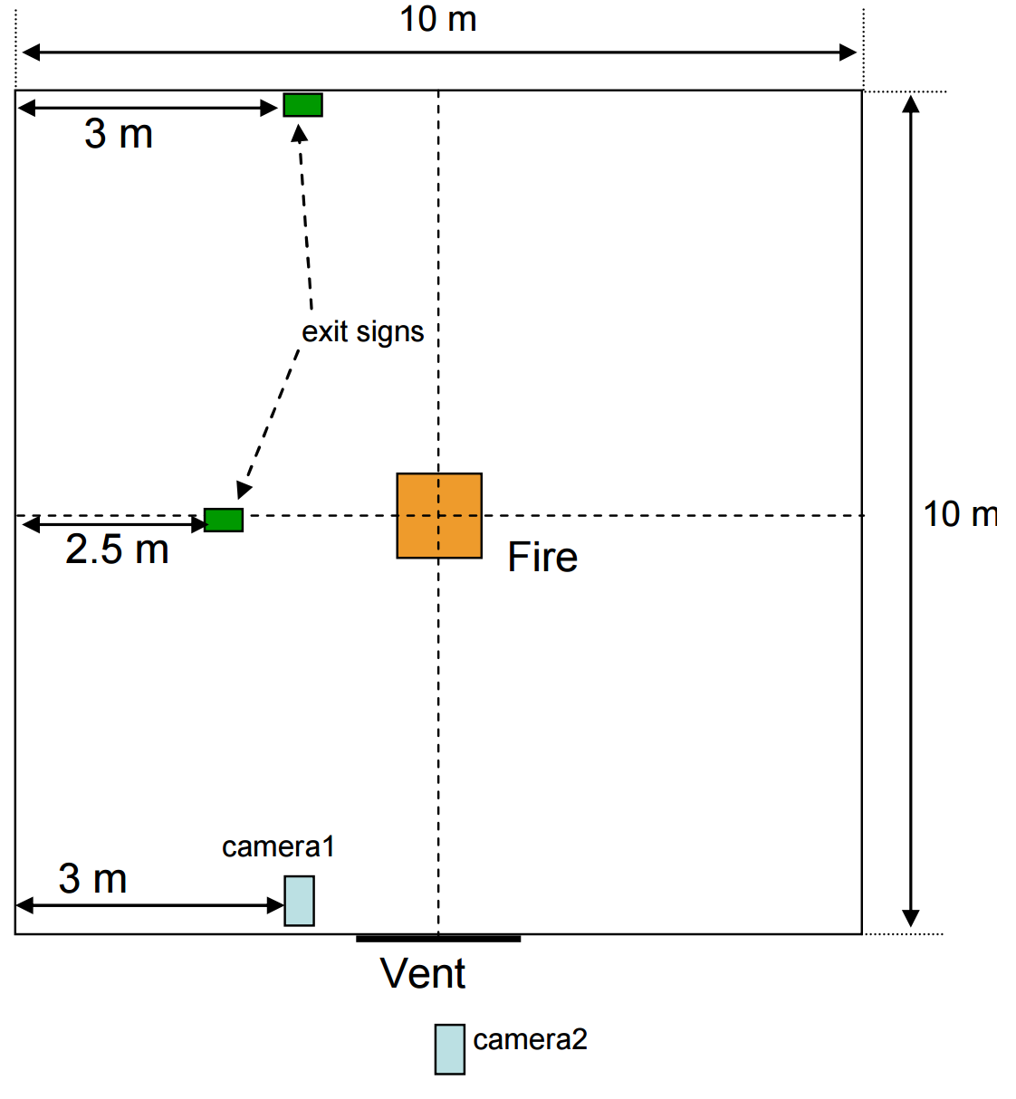
(Rinne, Hietaniemi, and Hostikka 2007) at the VTT Research Center of Finland performed a series of experiments to validate FDS simulations of smoke and toxic gas concentrations. These calculations were performed using version 4.05 of the Fire Dynamics Simulator (FDS). For this post, we repeated the calculation using FDS version 6.5.3. This model has previously been used in posts discussing fire modeling. In this post, we will focus on the smoke and visibility of the exit signs. Figure 6 and Figure 7 show side and top views of the experiment. 

For this study, we simulated the toluene fuel experiment, since that fuel provided experimental data to calculated smoke density. The experimentally measured peak HRR was 145.7 kW, which corresponds to a \(D^{*}\) = 0.444 m m. We changed the model to use multiple meshes with a cell size of 5 cm for the fire and opening. This gives a \(\frac{D^{*}}{\delta x}\) value of approximately 10, which should properly capture entrainment of air in the fire plume. 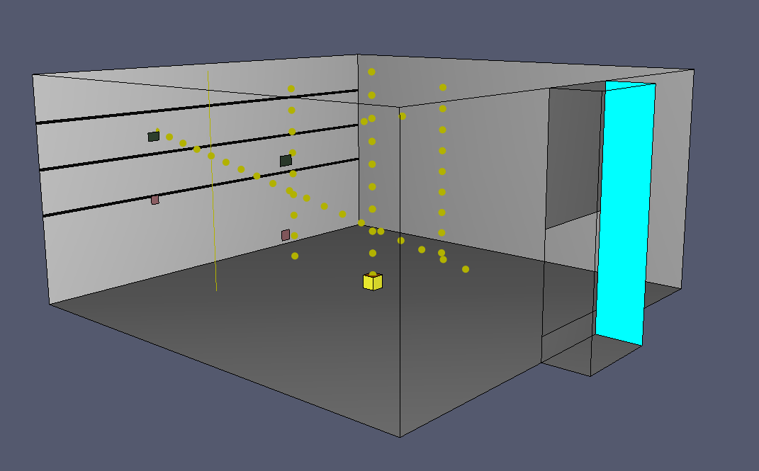The model is shown in Figure 8. The rgb values of the signs in the model were set to correspond to the rgb values measured from the initial camera image of the experiment. 

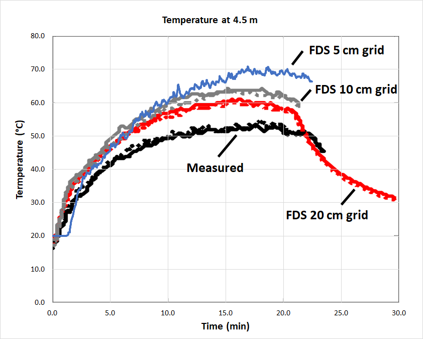
The original VTT paper gives results for 20 cm and 10 cm meshes. We give two representative graphs that compare results from the original study to the present study. Recall that changes include using FDS version 6.5.3 (version 4.05 in original) and refining the mesh. Figure 9 shows the temperature at a height of 4.5 m. The measure experimental results and the model results are essentially identical for both of the thermocouple trees. 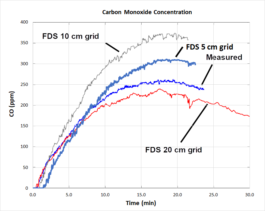Figure 10 compares the \(CO\) concentration. Figure 11 compares smoke layer height, which is extracted in FDS using the temperature profile as a function of height. The smoke layer results for the 5 cm case are 10 to 20 cm lower than when measured experimentally.

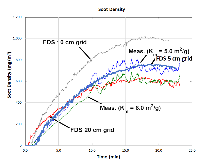
To compare the visibility and obscuration due to smoke, we can first compare the experimentally measured soot density to the FDS results, Figure 12. The reader is referred to the VTT paper for a full description of the density measurement, but the procedure used equations 1, 2, and 3 to convert light transmission measurements made with a MIREX device to density by calculating the mass specific extinction coefficient as a function of wavelength. As can be seen, the 5 cm results fall within the experimental data range.

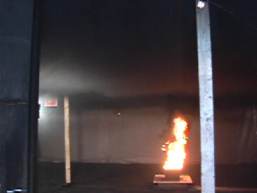
We can also make a direct comparison with an image taken by a camera located just outside the vent opening. Figure 13 shows the picture at 6 minutes. This can be compared to the PyroSim image in Figure 14, which displays a slightly lower layer of smoke. We can also see that interior lighting was included in the experiment that helped illuminate the exit sign. As shown by the red hue on the bottom of the smoke layer, the fire also contributed to lighting.

5. Summary

In this post we have accomplished three things:

Although there are several uncertainties in the calculation of soot density and the conversion of the density to visibility and obscuration, the comparison of VTT experimental images with predicted smoke visualization for the toluene fuel shows remarkably good correlation (Figure 13 and Figure 14). It should be noted that the VTT paper indicates that the predicted obscuration was greater than observed for wood and PMMA fires.

We expect that future development of the results visualization in PyroSim will include options to incorporate interior lights and fire illumination.

6. Miscellaneous Comments

One initial source of confusion for me was the difference between the thermal radiation calculation and the visibility/obscuration calculation. The calculation of thermal radiation in the energy equation is completely independent of the visibility and obscuration calculation, Section 2.6.2 of FDS Technical Reference Guide (McGrattan et al. 2019). The default thermal radiation calculation assumes a gray gas model where the radiation absorption coefficient is calculated using the RadCal program. This is similar to the Planck mean absorption coefficient calculated by (Widmann 2003) by integrating over all wavelengths.

To download the most recent version of PyroSim, please visit the the PyroSim Support page and click the link for the current release. If you have any questions, please contact support@thunderheadeng.com.

7. Bibliography

Forney, Glenn. 2019. Smokeview, A Tool for Visualizing Fire Dynamics Simulation Data Volume III: Verification Guide, NIST Special Publication 1017-3. Sixth Edition. National Institute of Standards and Technology, Gaithersburg, Maryland, USA: NIST.

Gross, R., J.J. Loftus, and A.F. Robertson. 1966. “Method for Measuring Smoke from Burning Materials.” https://doi.org/10.1520/STP41310S.

Jin, T. 1997. “Studies on Human Behavior and Tenability in Fire Smoke.” Fire Safety Science. https://doi.org/10.3801/IAFSS.FSS.5-3.

al., Kevin McGrattan et. 2019. Fire Dynamics Simulator Technical Reference Guide Volume 2: Verification, NIST Special Publication 1018-2. Sixth Edition. National Institute of Standards and Technology, Gaithersburg, Maryland, USA: NIST.

McGrattan, Kevin, Simo Hostikka, Randall McDermott, Jason Floyd, and Marcos Vanella. 2021. Fire Dynamics Simulator User’s Guide, NIST Special Publication 1019. Sixth Edition. National Institute of Standards and Technology, Gaithersburg, Maryland, USA: NIST.

Mulholland, George W., and Carroll Croarkin. 2000. “Specific Extinction Coefficient of Flame Generated Smoke.” Fire and Materials 24 (5): 227–30. https://doi.org/10.1002/1099-1018(200009/10)24:5<227::AID-FAM742>3.0.CO;2-9.

Rinne, Tuomo, Jukka Hietaniemi, and Simo Hostikka. 2007. “Experimental Validation of the FDS Simulations of Smoke and Toxic Gas Concentrations.”

SFPE. 2016. SFPE Handbook of Fire Protection Engineering. 5th ed. Springer-Verlag New York. https://www.springer.com/us/book/9781493925643.

Widmann, John. 2003. “Evaluation of the Planck Mean Absorption Coefficients for Radiation Transport through Smoke.” Combustion Science and Technology - COMBUST SCI TECHNOL 175 (December): 2299–2308. https://doi.org/10.1080/714923279.