Modeling Jet Fans

Reading Time: 28 minutes

Created with software version: 2020.1

To follow along with this tutorial, download the relevant files here.

1. Introduction

This tutorial discusses modeling jet fans using FDS/PyroSim, with the eventual goal of modeling parking garages. It starts with some background information that is useful in helping understand the problem. In preparation for a parking garage simulation, we first focus on a free jet, comparing the results of a mesh convergence study with the experimentally derived correlations for centerline velocity decay. This tutorial should help you decide whether PyroSim is applicable to your jet fan application.

FDS (the Fire Dynamics Simulator developed at NIST), the backend of PyroSim, solves the Navier-Stokes equations using the Large Eddy Simulation (LES) method. In the LES approach, eddies on the scale of the cell size are resolved and the effect of smaller eddies are approximated. This means that the solution is transient and will vary with time at any point. In contrast, the Reynolds Averaged Navier-Stokes (RANS) approach provides a single time averaged solution.

As will be demonstrated, the mesh size required to accurately match the experimental data for a free jet from a duct are smaller than can be realistically incorporated in a typical design application, such as a parking garage. The question then becomes, “Are there approaches that allow us to reasonably simulate a jet fan in a design calculation, while still being able to solve the problem in realistic time frames?” In the next section we will attempt to provide some guidance to this issue.

In this section we simulate a free air jet with increasing mesh resolution to validate that the FDS solution does converge to the experimental data as mesh is refined.

2. Background and Convergence Study

2.1. Jet Fan Backgound

Several papers help begin to understand some of the issues in modeling jet fans. This is far from an exhaustive list, but it at least provides a starting point for our discussion:

Modelling and simulation of a jet fan for controlled air flow in large enclosures, (v.d.Giesen et al. 2011) describes both experiments and a RANS computational fluid dynamics (CFD) simulation. The goal is to model the experiments described in this paper.
Hazim Awbi’s book on Ventilation of Buildings (Awbi 2003) is one source for a background discussion of experimental data and equations that fit the data.
Two papers, Numerical Study on Impulse Ventilation for Smoke Control in an Underground Car Park (Lu et al. 2011) and The use of impulse ventilation for smoke control in underground car parks (Viegas 2010) demonstrate detailed simulation of ventilation for smoke control in underground car parks using FDS.
The NIST verification manual for FDS includes a jet fan calculation and references correlations with experimental data (McGrattan 2020).

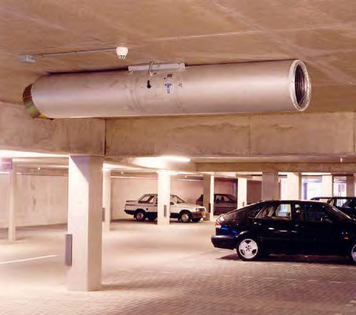
A typical jet fan installation in a parking facility is shown. Brochures from manufacturers, such as the FANTECH catalog Impulse Ventilation for Car Parks, provide possible arrangements of arrays of fans in application.

irl jet fan installation — Figure 1. Typical jet fan installation (v.d.Giesen et al. 2011)

A free air jet flows into an air space where there are no solid boundaries to influence the flow pattern. As described by Awbi (Awbi 2003) the flow from a free circular jet can be divided into two regions:

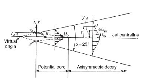
doc scrn jet circular jet schematic — Figure 2. Schematic of a free circular jet (Awbi 2003)

Potential core region is the region immediately downstream of the supply opening where mixing of the jet fluid with the surrounding fluid is not complete. The length of the core … usually extends to 5-10 equivalent opening diameters. In this region the centerline velocity is constant and equal to the supply velocity.
Axisymmetric decay region is a region dominated by a highly turbulent flow generated by viscous shear at the edge of the shear layer. For three-dimensional jets this is usually referred to as the ‘fully developed flow region’ where the spread angle of the jet is a constant whose value depends on the geometry of the opening. It is the predominant region for a jet discharging from a low aspect ratio (square or circular) opening where it extends to about 100 equivalent diameters. Centerline velocity decreases inversely with the distance from the opening.
(Awbi 2003)

As described by Awbi (Awbi 2003), Baturin (Baturin 1972) provides the following fit to experimental data:

Baturin Equation

\[u_{m}\left( x \right) = \frac{0.48}{\left( ax/d_{0} + 0.145 \right)}\times u_{0}\]

Where:

\(u_{m}\) is the centerline velocity.
\(u_{0}\) is the supply velocity.
\(x\) is distance from the supply.
\(a\) is a constant (0.076 to 0.080 for cylindrical tubes).
\(d_{0}\) is the supply diameter.

Another representation of jet fan experimental data is provided by Kümmel (Eck 2007) and is described in the FDS Verification Guide (McGrattan 2020).

For a Square Duct

\[x_0 = \frac{h}{m}\]

Kümmel Equation

\[u_{m}(x)=\frac{x_{0}}{x}\]

Where:

\(x_{0}\) is the length of the potential core.
\(h\) is the side length of the square duct.
\(m\) is a constant that varies between 0.12 and 0.20.

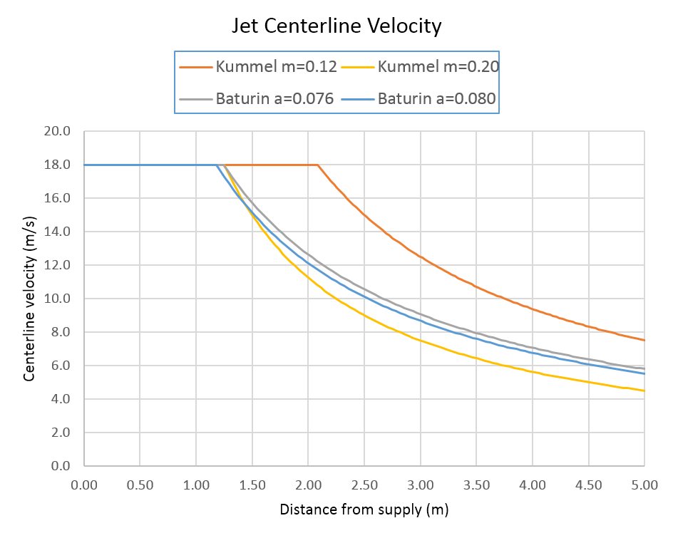
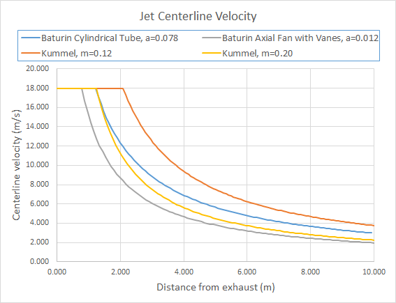
The Baturin and Kümmel equations are displayed below for a square 0.25 m duct (equivalent diameter 0.2821 m) with an initial air velocity of 18 m/s (= 59.1 ft/s = 64.8 km/hr = 40.2 miles/hr), and the outlet velocity of the jet fan in the Giesen et al., 2011 paper (v.d.Giesen et al. 2011). The bounds of the Kümmel equation show a significant variation in the length of the potential core region. The Baturin correlation predicts centerline velocities that lie between the bounds of the Kümmel predictions. When comparing the PyroSim/FDS results with the correlations, the mean values of the Baturin and Kümmel equation parameters are used.

plot graph jet centerline velocities — Figure 3. Analytic free jet centerline velocities.

2.2. FDS Simulation of Free Jet

Before proceeding to simulate the parking garage experiment, we will simulate a free jet using varying mesh refinements. The model consists of a 0.25 m x 0.25 m vent with a supply velocity of 18 m/s, similar to the jet fan dimensions and performance that was tested by Giesen et al. (v.d.Giesen et al. 2011).

Figure 4 shows the free jet model. Five meshes were used, with the boundaries of each mesh being an X length of 2.5 m and a height and width of 1.25 m. Only a single mesh is used near the vent, but four meshes are used away from the vent, since the diameter of the jet increases with distance from the supply vent.

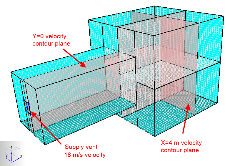
pyro scrn jet model — Figure 4. The free jet model. The total X length is 5 m.

excel scrn jet fan mesh size — Figure 5. Jet Fan Mesh Size

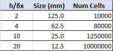
The supply vent was square with each side length \(h\) = 0.25 m and with a supply velocity of 18 m/s. The cell size (δx) was equal in X, Y, and Z and was varied as a fraction of the vent side dimension, as shown in the table. The number of cells in the models ranged from 10x10³ to 10x10⁶.

2.3. Results of FDS Free Jet Simulations

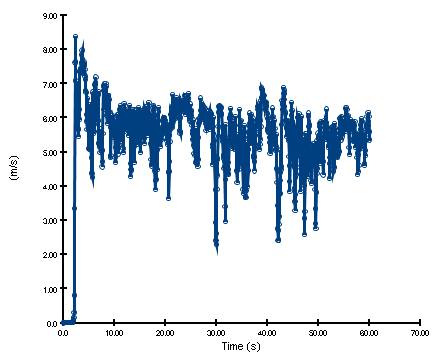
Because FDS is a Large Eddy Simulation (LES) solution, the results vary with time. All models were run for 10 s. The initial transient is complete by 2 s and the primary turbulence frequencies are sufficiently high that averaging the results from 2 s to 10 s gives a value that represents a steady state measurement. The previous figure shows the locations of the Y = 0 m and X = 4 m planes on which velocity contours will be presented.

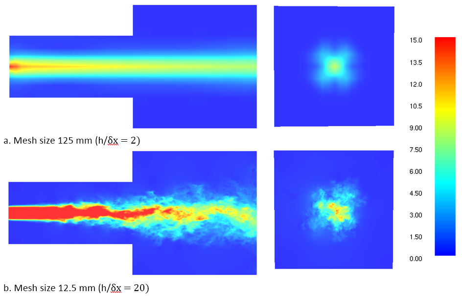
To first visualize the effect of mesh size on the solution, we present two pairs of velocity contours on the Y = 0 m and X = 4 m planes at 5 s. These provide both a sense of how the mesh captures turbulence and a measure of the size of the downstream jet. Clearly, the fine mesh shows a much more realistic development of the shear layer, while the coarse mesh result shows minimal turbulence.

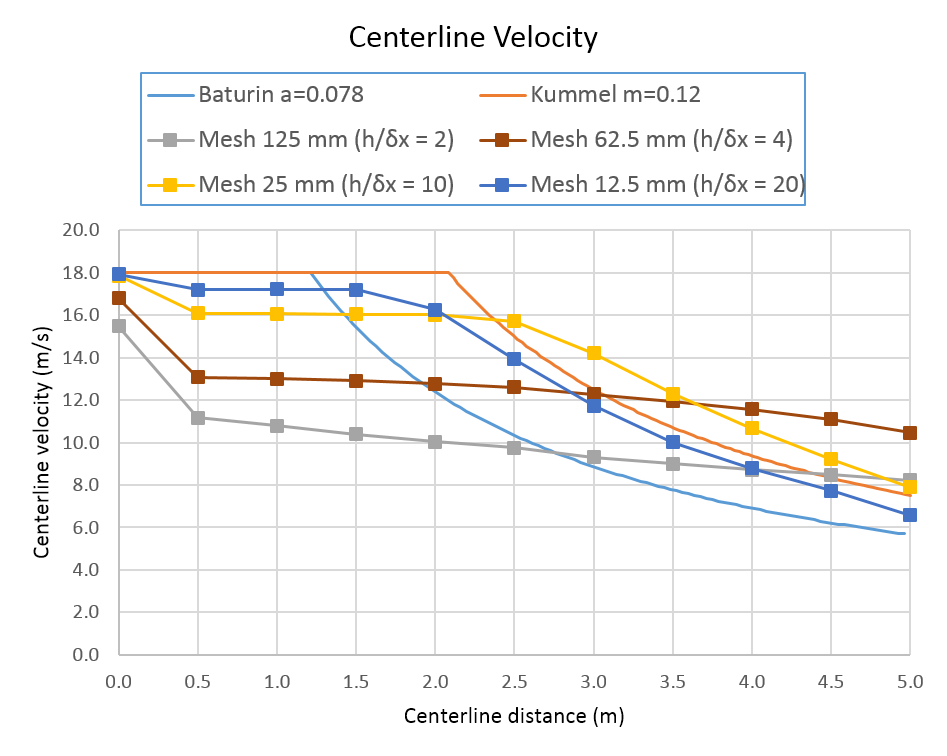
results scrn jet fan velocity contours — Figure 6. Free jet velocity contours. The left column shows velocity on the Y = 0 plane (0 ≤ X ≤ 5 m). The right column shows the contours on the X = 4 m plane. The velocity color bars bounds are 0 and 15 m/s, with values above 15 m/s drawn in red.

A comparison of the calculated centerline velocities with the analytic correlations is shown below. Again we see that a fine mesh is required to capture the velocity decay within the 5 m of the outlet. The fine mesh where the grid size is 1/20 of the outlet vent side provides reasonable results.

plot graph jet fan centerline velocities — Figure 7. Calculated free jet centerline velocities.

2.4. Summary

If a sufficiently refined mesh is used, FDS can accurately simulate a free jet. If the mesh refinement is too coarse, the solution will not capture the turbulence in the shear layer that entrains the surrounding fluid and the predicted centerline velocity will not decay as shown be experiment.

This is similar to the conclusion in the FDS Verification Manual, where a mesh of 1/16 the vent side was needed to obtain an reasonably accurate solution. The FDS Verification Manual free jet test problem has a Reynolds number of 1x10⁵ (square duct side 0.8 m and a fluid velocity of 2 m/s). The parameters of the free jet in this section are more challenging and were chosen to approximate a commercial jet fan used for parking garages with a Reynolds number of 2.7x10⁵ (square duct side 0.25 m and a fluid velocity of 18 m/s). So the duct size is significantly smaller and the fluid velocity is significantly higher.

In the next section we will explore ways to speed the solution while still obtaining reasonable results.

2.5. FDS Input File Listing

&free jet 0_0125 for post.fds
&Generated by PyroSim - Version 2014.4.1208
&Feb 16, 2015 2:48:26 PM

&HEAD CHID='free_jet_0_0125_for_post'/
&TIME T_END=10.0/
&DUMP RENDER_FILE='free_jet_0_0125_for_post.ge1', DT_RESTART=2.5/

&MESH ID='Mesh-a-e', IJK=200,100,100, XB=0.0,2.5,-0.625,0.625,-0.625,0.625/
&MESH ID='Mesh-b-a', IJK=200,100,100, XB=2.5,5.0,-1.25,-1.11022E-15,-1.25,-1.11022E-15/
&MESH ID='Mesh-b-b', IJK=200,100,100, XB=2.5,5.0,-1.25,-1.11022E-15,-1.11022E-15,1.25/
&MESH ID='Mesh-b-c', IJK=200,100,100, XB=2.5,5.0,-1.11022E-15,1.25,-1.25,-1.11022E-15/
&MESH ID='Mesh-b-d', IJK=200,100,100, XB=2.5,5.0,-1.11022E-15,1.25,-1.11022E-15,1.25/

&DEVC ID='Vel x0_0 z0_000', QUANTITY='VELOCITY', XYZ=0.0125,0.0,0.0, ORIENTATION=1.0,0.0,0.0/
&DEVC ID='Vel x0_5 z0_000', QUANTITY='VELOCITY', XYZ=0.5,0.0,0.0, ORIENTATION=1.0,0.0,0.0/
&DEVC ID='Vel x1_0 z0_000', QUANTITY='VELOCITY', XYZ=1.0,0.0,0.0, ORIENTATION=1.0,0.0,0.0/
&DEVC ID='Vel x1_5 z0_000', QUANTITY='VELOCITY', XYZ=1.5,0.0,0.0, ORIENTATION=1.0,0.0,0.0/
&DEVC ID='Vel x2_0 z0_000', QUANTITY='VELOCITY', XYZ=2.0,0.0,0.0, ORIENTATION=1.0,0.0,0.0/
&DEVC ID='Vel x2_5 z0_000', QUANTITY='VELOCITY', XYZ=2.5,0.0,0.0, ORIENTATION=1.0,0.0,0.0/
&DEVC ID='Vel x3_0 z0_000', QUANTITY='VELOCITY', XYZ=3.0,0.0,0.0, ORIENTATION=1.0,0.0,0.0/
&DEVC ID='Vel x3_5 z0_000', QUANTITY='VELOCITY', XYZ=3.5,0.0,0.0, ORIENTATION=1.0,0.0,0.0/
&DEVC ID='Vel x4_0 z0_000', QUANTITY='VELOCITY', XYZ=4.0,0.0,0.0, ORIENTATION=1.0,0.0,0.0/
&DEVC ID='Vel x4_5 z0_000', QUANTITY='VELOCITY', XYZ=4.5,0.0,0.0, ORIENTATION=1.0,0.0,0.0/
&DEVC ID='Vel x5_0 z0_000', QUANTITY='VELOCITY', XYZ=5.0,0.0,0.0, ORIENTATION=1.0,0.0,0.0/
&SURF ID='Vent Supply',
RGB=26,204,26,
VEL=-18.0/

&VENT SURF_ID='OPEN', XB=0.0,0.0,0.125,0.625,-0.625,0.625/ Mesh Vent: Mesh-a-e [XMIN]
&VENT SURF_ID='OPEN', XB=0.0,2.5,0.625,0.625,-0.625,0.625/ Mesh Vent: Mesh-a-e [YMAX]
&VENT SURF_ID='OPEN', XB=0.0,2.5,-0.625,-0.625,-0.625,0.625/ Mesh Vent: Mesh-a-e [YMIN]
&VENT SURF_ID='OPEN', XB=0.0,2.5,-0.625,0.625,0.625,0.625/ Mesh Vent: Mesh-a-e [ZMAX]
&VENT SURF_ID='OPEN', XB=0.0,2.5,-0.625,0.625,-0.625,-0.625/ Mesh Vent: Mesh-a-e [ZMIN]
&VENT SURF_ID='OPEN', XB=0.0,0.0,-0.625,-0.125,-0.625,0.625/ Mesh Vent: Mesh-a-e [XMIN]01
&VENT SURF_ID='OPEN', XB=0.0,0.0,-0.125,0.125,0.125,0.625/ Mesh Vent: Mesh-a-e [XMIN]02
&VENT SURF_ID='OPEN', XB=0.0,0.0,-0.125,0.125,-0.625,-0.125/ Mesh Vent: Mesh-a-e [XMIN]03
&VENT SURF_ID='OPEN', XB=5.0,5.0,-1.25,-1.11022E-15,-1.25,-1.11022E-15/ Mesh Vent: Mesh-b-a [XMAX]
&VENT SURF_ID='OPEN', XB=2.5,2.5,-0.625,-1.11022E-15,-1.25,-0.625/ Mesh Vent: Mesh-b-a [XMIN]
&VENT SURF_ID='OPEN', XB=2.5,2.5,-1.25,-0.625,-1.25,-1.11022E-15/ Mesh Vent: Mesh-b-a [XMIN]
&VENT SURF_ID='OPEN', XB=2.5,5.0,-1.25,-1.25,-1.25,-1.11022E-15/ Mesh Vent: Mesh-b-a [YMIN]
&VENT SURF_ID='OPEN', XB=2.5,5.0,-1.25,-1.11022E-15,-1.25,-1.25/ Mesh Vent: Mesh-b-a [ZMIN]
&VENT SURF_ID='OPEN', XB=5.0,5.0,-1.25,-1.11022E-15,-1.11022E-15,1.25/ Mesh Vent: Mesh-b-b [XMAX]
&VENT SURF_ID='OPEN', XB=2.5,2.5,-1.25,-0.625,-1.11022E-15,1.25/ Mesh Vent: Mesh-b-b [XMIN]
&VENT SURF_ID='OPEN', XB=2.5,2.5,-0.625,-1.11022E-15,0.625,1.25/ Mesh Vent: Mesh-b-b [XMIN]
&VENT SURF_ID='OPEN', XB=2.5,5.0,-1.25,-1.25,-1.11022E-15,1.25/ Mesh Vent: Mesh-b-b [YMIN]
&VENT SURF_ID='OPEN', XB=2.5,5.0,-1.25,-1.11022E-15,1.25,1.25/ Mesh Vent: Mesh-b-b [ZMAX]
&VENT SURF_ID='OPEN', XB=5.0,5.0,-1.11022E-15,1.25,-1.25,-1.11022E-15/ Mesh Vent: Mesh-b-c [XMAX]
&VENT SURF_ID='OPEN', XB=2.5,2.5,-1.11022E-15,0.625,-1.25,-0.625/ Mesh Vent: Mesh-b-c [XMIN]
&VENT SURF_ID='OPEN', XB=2.5,2.5,0.625,1.25,-1.25,-1.11022E-15/ Mesh Vent: Mesh-b-c [XMIN]
&VENT SURF_ID='OPEN', XB=2.5,5.0,1.25,1.25,-1.25,-1.11022E-15/ Mesh Vent: Mesh-b-c [YMAX]
&VENT SURF_ID='OPEN', XB=2.5,5.0,-1.11022E-15,1.25,-1.25,-1.25/ Mesh Vent: Mesh-b-c [ZMIN]
&VENT SURF_ID='OPEN', XB=5.0,5.0,-1.11022E-15,1.25,-1.11022E-15,1.25/ Mesh Vent: Mesh-b-d [XMAX]
&VENT SURF_ID='OPEN', XB=2.5,2.5,-1.11022E-15,0.625,0.625,1.25/ Mesh Vent: Mesh-b-d [XMIN]
&VENT SURF_ID='OPEN', XB=2.5,2.5,0.625,1.25,-1.11022E-15,1.25/ Mesh Vent: Mesh-b-d [XMIN]
&VENT SURF_ID='OPEN', XB=2.5,5.0,1.25,1.25,-1.11022E-15,1.25/ Mesh Vent: Mesh-b-d [YMAX]
&VENT SURF_ID='OPEN', XB=2.5,5.0,-1.11022E-15,1.25,1.25,1.25/ Mesh Vent: Mesh-b-d [ZMAX]
&VENT SURF_ID='Vent Supply', XB=0.0,0.0,-0.125,0.125,-0.125,0.125/ Vent

&ISOF QUANTITY='VELOCITY', VALUE=1.0,2.0,5.0,10.0,15.0/

&SLCF QUANTITY='VELOCITY', VECTOR=.TRUE., PBX=0.25/
&SLCF QUANTITY='VELOCITY', VECTOR=.TRUE., PBX=0.5/
&SLCF QUANTITY='VELOCITY', VECTOR=.TRUE., PBX=1.0/
&SLCF QUANTITY='VELOCITY', VECTOR=.TRUE., PBX=1.5/
&SLCF QUANTITY='VELOCITY', VECTOR=.TRUE., PBX=2.0/
&SLCF QUANTITY='VELOCITY', VECTOR=.TRUE., PBX=3.0/
&SLCF QUANTITY='VELOCITY', VECTOR=.TRUE., PBX=4.0/
&SLCF QUANTITY='VELOCITY', VECTOR=.TRUE., PBX=5.0/
&SLCF QUANTITY='VELOCITY', VECTOR=.TRUE., PBY=0.0/
&SLCF QUANTITY='VELOCITY', VECTOR=.TRUE., PBZ=0.0/

&DEVC ID='[Species: AIR] Mass Flux X=1.0_AREA INTEGRAL', QUANTITY='MASS FLUX X', SPEC_ID='AIR', STATISTICS='AREA INTEGRAL', XB=1.0,1.0,-0.625,0.625,-0.625,0.625/
&DEVC ID='[Species: AIR] Mass Flux X=2.0_AREA INTEGRAL', QUANTITY='MASS FLUX X', SPEC_ID='AIR', STATISTICS='AREA INTEGRAL', XB=2.0,2.0,-0.625,0.625,-0.625,0.625/
&DEVC ID='[Species: AIR] Mass Flux X=3.0_AREA INTEGRAL', QUANTITY='MASS FLUX X', SPEC_ID='AIR', STATISTICS='AREA INTEGRAL', XB=3.0,3.0,0.0,1.25,0.0,1.25/
&DEVC ID='[Species: AIR] Mass Flux X=4.0_AREA INTEGRAL', QUANTITY='MASS FLUX X', SPEC_ID='AIR', STATISTICS='AREA INTEGRAL', XB=4.0,4.0,0.0,1.25,0.0,1.25/
&DEVC ID='[Species: AIR] Mass Flux X=5.0_AREA INTEGRAL', QUANTITY='MASS FLUX X', SPEC_ID='AIR', STATISTICS='AREA INTEGRAL', XB=5.0,5.0,0.0,1.25,0.0,1.25/

&TAIL /

3. Validation Using Experimental Data

We will now explore two approaches to modeling jet fans using FDS:

Velocity Patches.
HVAC Ducts.

For the velocity patch we examine the effects of different shroud lengths, and for the HVAC duct we examine the effects of a short downstream shroud. We evaluate the models using the downstream centerline velocity and flow entrainment.

In Chapter 2 we did a quick background review of downstream flow, including the Potential core and Axisymmetric decay regions for a free circular jet. In this section we will focus on modeling the Novenco jet fan tested by Giesen et al. (v.d.Giesen et al. 2011): with diameter 290 mm, length 2.6 m, exhaust flow rate 1.0 m³/s, exhaust air velocity 18 m/s = 59.1 ft/s = 64.8 km/hr = 40.2 miles/hr, capacity 21 N. For flow conditions that represent this fan, Chapter 2 found that a mesh size of 12.5 mm was required to obtain reasonably accurate results for the first 5 m downstream of the outlet. Unfortunately, it is not feasible to simulate full scale parking garages with such a fine mesh, even if multiple meshes are used, so in this section we examine alternate approaches.

3.1. Background Equations for Jet Fans

Both the Kümmel and Baturin equations listed in Chapter 2 are plotted below for a square 0.25 m square duct (equivalent diameter 0.2821 m) with an initial air velocity of 18 m/s. As will be discussed below, the Kummel equation with \(m\) = 0.20 provides a good match with jet fan results measured by Geiesen et al. (v.d.Giesen et al. 2011).

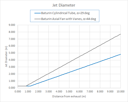
plot graph jet fan centerline eqs — Figure 8. Plots of the experimental correlations for the range of equation parameters.

Baturin also provides data on the spread angle for different jets. For a cylindrical tube \(\alpha\) = 29 deg and for an axial fan with guide vanes \(\alpha\) = 44 deg. The calculated jet diameters are shown in Figure 9.

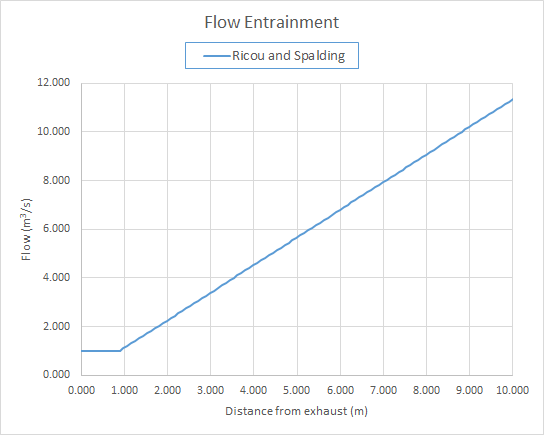
plot graph jet fan diameter — Figure 9. Plot of the jet diameter base on the Baturin equation. The value alpha is the total spread angle of the jet.

Ricou and Spalding (Ricou and Spalding 1961) developed the following expression for flow entrainment based on experimental measurements.

Ricou Equation

\[Q \left(x \right) = 0.32 \left( \frac{x}{d_0} \right) \times Q_0\]

Where:

\(Q\) is the volume flow rate at distance \(x\)
\(Q_{0}\) is the supply flow rate. This is plotted in Figure 10 for \(Q_{0}\) = 1 m³/s

plot graph jet flow entrainment — Figure 10. Flow entrainment based on experimental fit by Ricou and Spalding

3.2. Jet Fan Convergence Study

To model a jet fan, we must couple the inlet flow to the outlet while preserving the fuel, air, and product mixture. The jet fan in this convergence study is 1 m long and is a square duct with sides \(\alpha\) = 0.25 m and an outlet air velocity of 18 m/s. This test problem is similar to that in Chapter 2, except now we explicitly model the fan (not just a supply vent) and the centerline distance is extended to 10 m downstream of the fan. At 0.5 m intervals we use devices to measure the velocity time history.

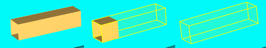
pyro scrn jet fan model — Figure 11. Jet fan simulation with 1 m long fan and 0.25 m sides. Distance from fan outlet to model boundary is 10 m.

3.3. Velocity Patch Model

In the Velocity Patch Tutorial, the fan is represented by a region where the axial (X) velocity is specified. The lateral (Y and Z) velocities are not defined. The velocity patch approach was implemented in FDS as an approach to approximate entrainment of air in sprinkler flow.

A velocity patch can be defined with or without a shroud surrounding the patch. The shroud (a hollow tube defined by thin obstructions) changes how adjacent air is drawn into the velocity patch and also focuses the flow in the axial direction of the shroud. For the convergence study, we explored three shroud configurations: full length shroud, short shroud (1/4 length), and no shroud.

pyro scrn jet velocity patch shrouds — Figure 12. Velocity patch shroud configurations (flow from left to right).

3.4. HVAC Model

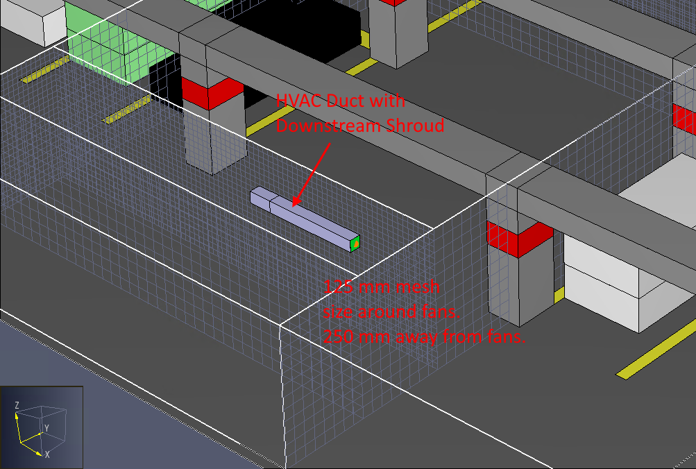
For the HVAC model, we used a standard HVAC duct with vents and a duct in which we used both an HVAC duct and a downstream shroud. We shorten the HVAC duct to 0.5 m and add a hollow shroud (similar to the velocity patch shroud) that extends downstream of the HVAC duct 0.5 m so that the length of the HVAC duct plus the shroud is equal to the total fan length.

The reason to add a shroud is to make sure the outlet flow is in the axial direction. FDS calculates cell velocities at the center of the cell sides (staggered grid). The HVAC duct is connected to the grid at a vent and the flow boundary conditions at the vent are specified on the faces of the cells that touch the vent. As a result, the flow can expand in the first cell downstream of the vent, reducing the axial velocity. This can be seen in the convergence study of Chapter 2. The shroud maintains the outlet flow in the axial direction, ensuring that the one dimensional axial velocity is preserved at the fan outlet.

3.5. Results of Convergence Study

The convergence study used the two with mesh sizes of 125 mm, 62.5 mm, and 31.25 mm. Since the jet fan side is 250 mm, these correspond to 2, 4, and 8 divisions along each side.

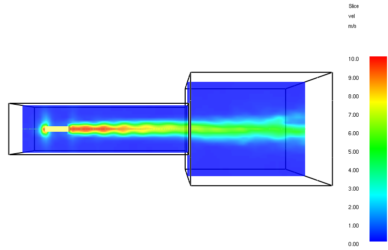
The figure below shows typical velocity contours for the standard HVAC model with a 125 mm mesh.

results jet fan hvac contours — Figure 13. Velocity contours for the standard HVAC duct model and a cell size of 125 mm.

And the figure below shows the measured velocities 7.5 m downstream of the outlet.

results scrn hvac 7.5m — Figure 14. The measured velocity time history 7.5 m downstream for the standard HVAC duct model and a cell size of 125 mm.

Results for the HVAC model are shown in Figure 15. For the HVAC model without a shroud, we see the initial lateral expansion of the flow at the outlet (blue lines in charts). All the results show less flow entrainment than the experimental fit, with the finer mesh of the shroud model having the closest match.

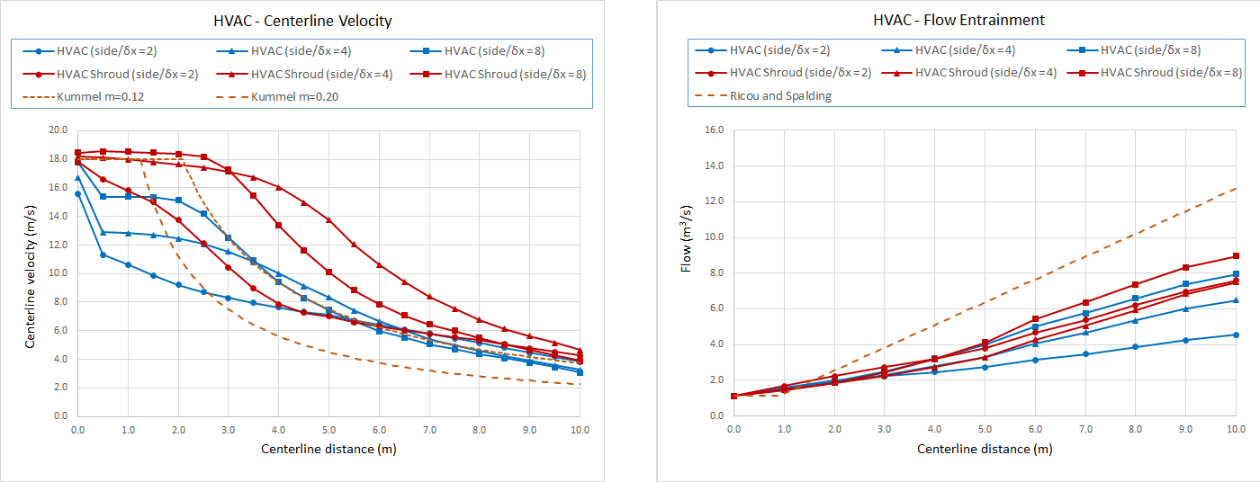
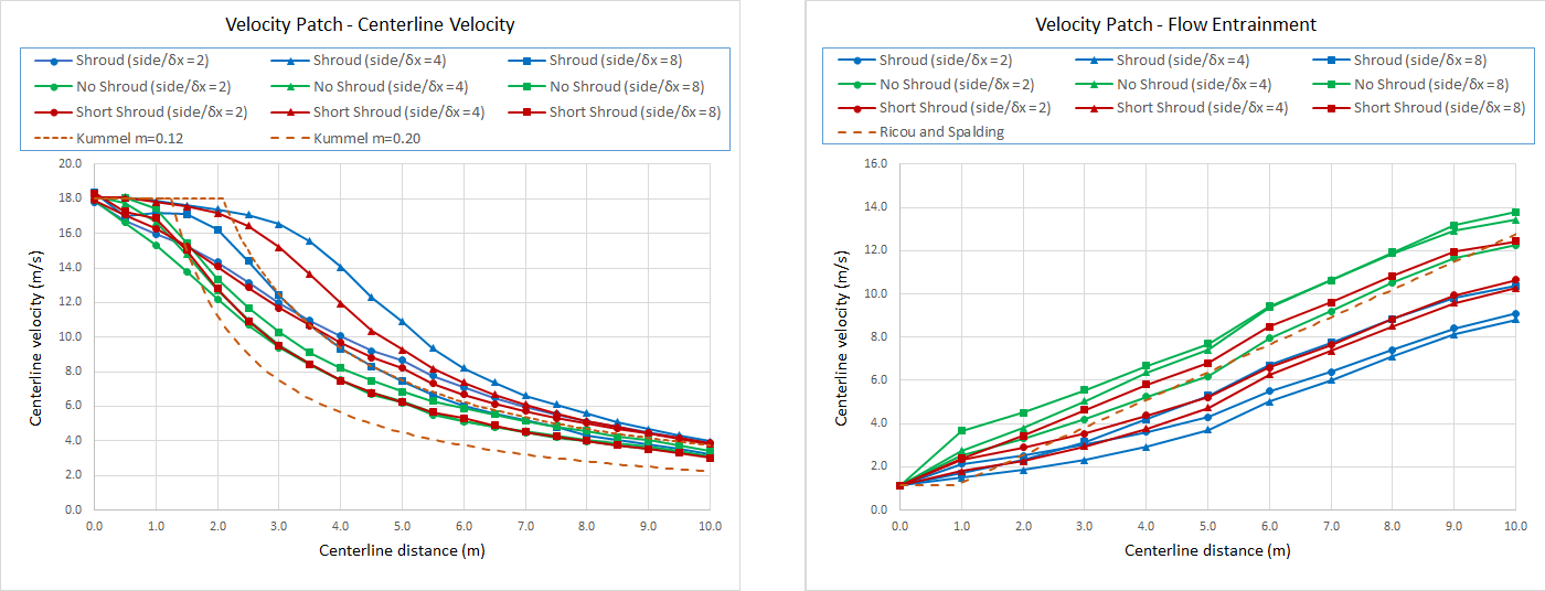
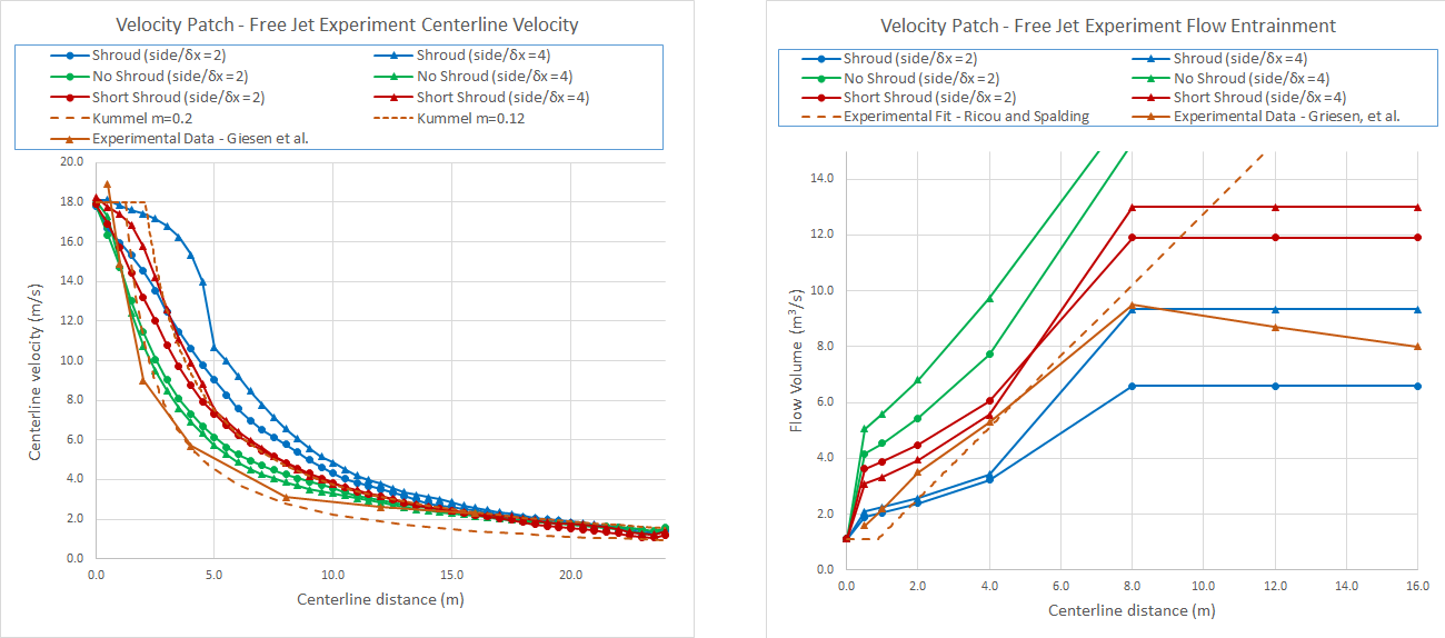
plot graph jet hvac convergence results 1 — Figure 15. Centerline velocity and flow entrainment for the convergence study using the HVAC duct model, with and without a downstream shroud.

Figure 16 shows the centerline velocity and flow entrainment for the convergence study for the jet fan model that used the velocity patch. For the centerline velocity, all the results approach the experimental fit at a downstream distance of 10 m. Closer to the jet fan outlet, the coarse mesh results (\(\delta x\) = 125 mm = side/2) undershoot the data, the medium mesh results (\(\delta x\) =62.5 mm = side/4) with a full or short shroud overshoot the data, and the fine mesh with the full shroud (\(\delta x\) =31.25 mm = side/8) matches the experimental fit quite well. The flow entrainment results show that reducing the shroud increases the flow, with no shroud the entrained flow is larger than desired.

plot graph jet velocity patch convergence — Figure 16. Centerline velocity and flow entrainment for the convergence study using the velocity patch model.

3.6. Geisen et al. Jet Fan Experiments

Geisen et al. (v.d.Giesen et al. 2011) describe jet fan experiments performed in a 34 m x 32 m x 6.5 m hall using a Novenco fan (diameter 290 mm, length 2.6 m, exhaust flow 1.0 m³/s, exhaust velocity 18 m/s, and capacity 21 N). Air velocity measurements were made at distances of 0.5 m, 1 m, 2 m, 4 m, 8 m, 12 m and 16 m from the exhaust. For the free jet experiment, the fan center was positioned 2.5 m above the floor.

The velocity profile at the exhaust from the actual fan is not uniform. An average velocity of 15.1 m/s is calculated using the stated fan diameter and flow, while a maximum centerline value of 18.9 m/s was measured in the experiments. In all the following calculations the fan outlet was assumed to be a 250 mm x 250 mm square with a velocity of 18 m/s (giving a flow of 1.125 m³/s).

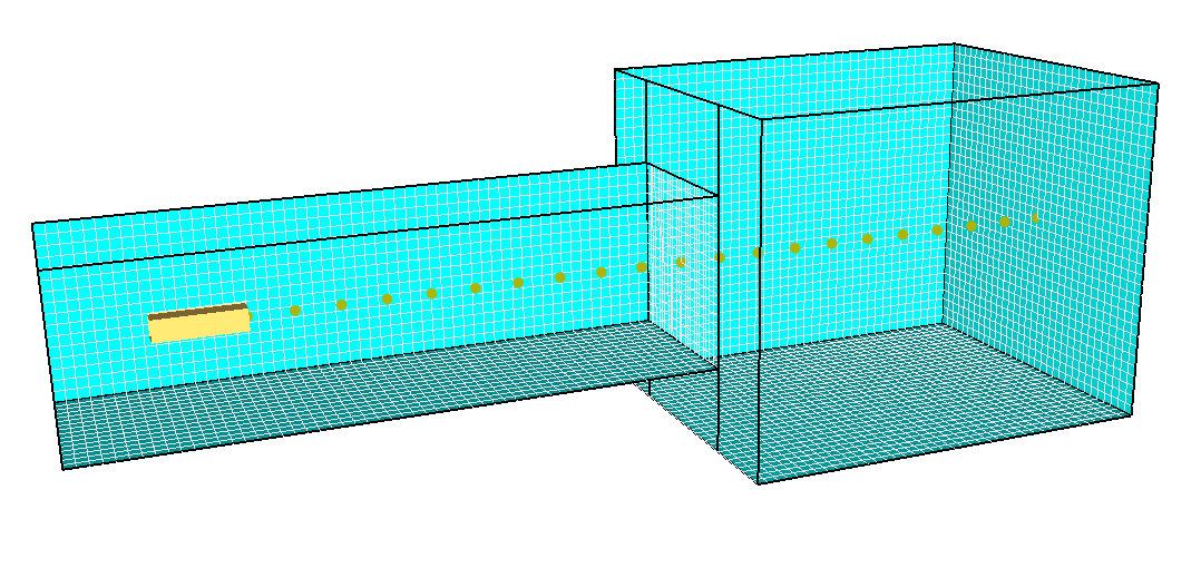
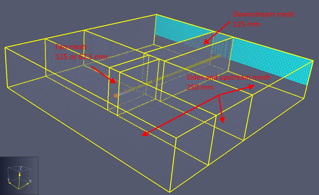
The jet fan experiment model is shown in Figure 17. As before, we model the jet fan using a velocity patch and an HVAC duct. At the fan, mesh resolutions of 125 mm and 62.5 mm were used, with 125 mm downstream and 250 mm on the sides of the fan. The upstream boundary was OPEN while the downstream boundary has a 2.3 m wall a distance of 24 m from the jet fan outlet.

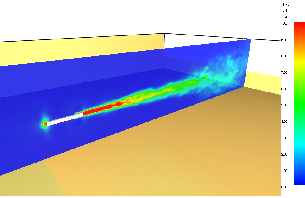
pyro scrn jet fan experiment mesh — Figure 17. The model used for the Geisen et al. experiment.

Velocity contours for the HVAC duct with a downstream shroud and mesh size 125 mm are shown below.

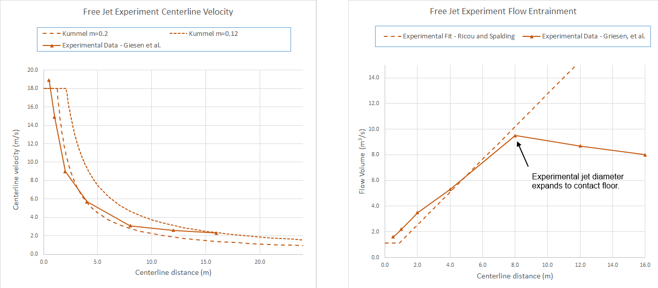
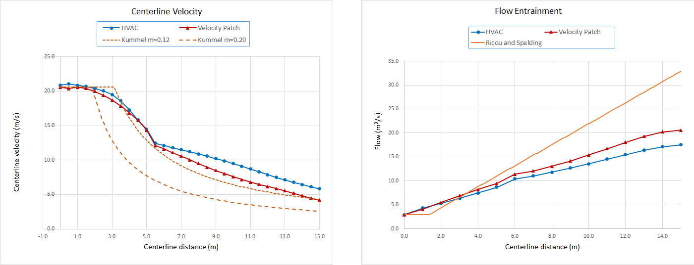
results scrn jet experiment velocity — Figure 18. Velocity contours for the HVAC duct with a downstream shroud and mesh size 125 mm.

First, we compare the Geisen et al. experimental measurements with the Kümmel (Eck 2007) equations. The experimentally measured centerline velocity shows good correlation with the Kümmel equation for \(m\) = 0.2. The experimentally measured flow entrainment matches the Ricou and Spalding equation until a downstream distance of about 8 m. At this point the diameter of the jet expands to where it interacts with the floor (the fan was mounted 2.5 m above the floor, so at a jet diameter of 5 m it has reached the floor). Referring to Figure 9, a jet diameter of 5 m is reached between 6.7 m and 10.2 m downstream, which corresponds to start of the plateau shown below.

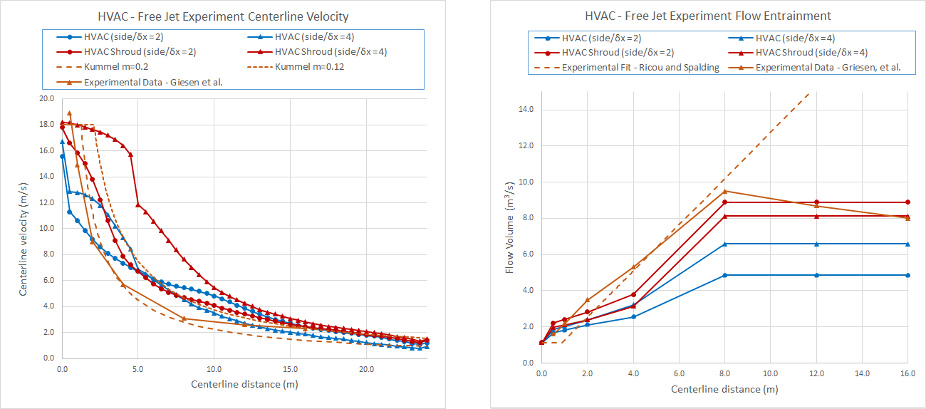
plot graph jet fan experiment results — Figure 19. Comparison of measured centerline velocity and flow entrainment for the Geisen et al. experiment with correlations.

Results for the HVAC model are shown in Figure 20. In this case, the HVAC duct with a downstream shroud and mesh size of 125 mm performed quite well in both matching the centerline velocity decay and the flow entrainment. This is an improved result compared to the convergence study.

plot graph jet hvac experiment results — Figure 20. Centerline velocity and flow entrainment for the Geisen et al. experiment using the HVAC duct model with and without a downstream shroud.

Results for the velocity patch model are shown in Figure 21. In general, the centerline velocity decay results are satisfactory, but for the No Shroud case the flow entrainment is much larger than measured and is not satisfactory. The short shroud with the coarse mesh is larger than the experimental fit by about 20%.

plot graph velocity patch results — Figure 21. Centerline velocity and flow entrainment for the Geisen et al. experiment using the velocity patch model.

3.7. Summary

There is no single model that was uniformly superior in both the convergence study and the modeling of the jet fan experiments.

Comparison with the experimental data of Geisen et al. (v.d.Giesen et al. 2011) shows that the HVAC duct with a downstream shroud and mesh size of 125 mm performed quite well in both matching the centerline velocity decay and the flow entrainment. The good news is that this is a feasible mesh size and the calculation uses the default FDS Deardorff turbulent viscosity model.

Alternately, the velocity patch model with the short shroud and mesh size of 125 mm had a better match with the flow entrainment for the convergence study and did a reasonable job for the experimental data.

4. Car Park Simulation

In this section, we demonstrate using FDS to model jet fans that extract smoke from a car park. The jet fans are modeled using the two approaches from Chapter 3. Two ventilation designs are presented: a design that did not perform satisfactorily and an improved design developed by James Allen at Fläkt Woods Group (james.allen@flaktwoods.com).

4.1. Application to Car Park

The purpose of this entire section is to demonstrate the feasibility of using FDS for jet fan simulations such as a car park. Based on what we have learned in Chapter 3, we will use a relatively coarse mesh with the jet fans modeled using HVAC ducts with downstream shrouds or velocity patches with short shrouds.

4.1.1. First Design

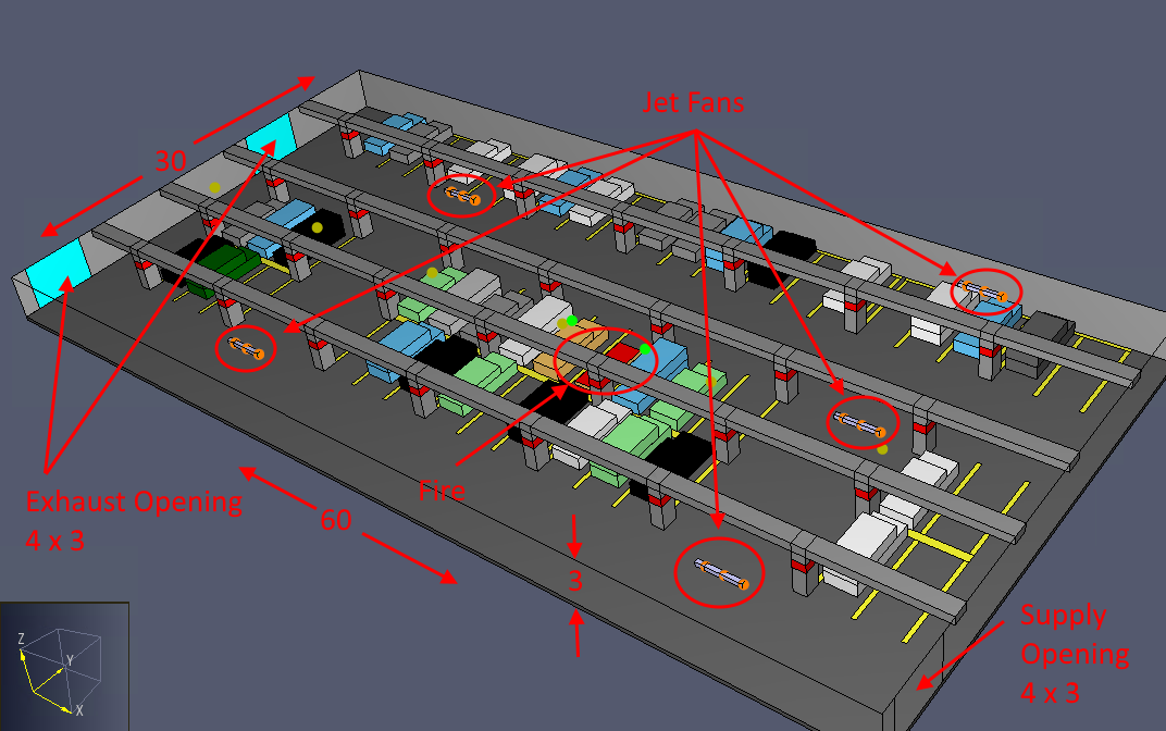
Figure 22 shows the basic car park dimensions and the first smoke control design that used five fans.

The total volume of the car park is 5400 m³. In the first design, there are two 4 m x 3 m exhaust openings and one 4 m x 3 m supply opening. The five fans (0.25 m x 0.25 m x 2.5 m) are arranged to direct the flow towards the exhaust openings. For 6 air changes per hour, the flow needs to be 9 m³/s or about 11 kg/s. We will present results for a case with a fan velocity of 18 m/s – the speed corresponding to the Novenco jet fan tested by Giesen et al. (v.d.Giesen et al. 2011). This case gives about a 30 kg/s replacement air flow (about 16 air changes per hour).

pyro scrn jet car park model — Figure 22. Car park model. Five fans in a 60x30x3 m garage.

The mesh size was 125 mm surrounding the fans and 250 mm away from the fans. Simple models of beams, columns, and cars were included.

pyro scrn jet car park fan — Figure 23. Detail of mesh around HVAC jet fan duct.

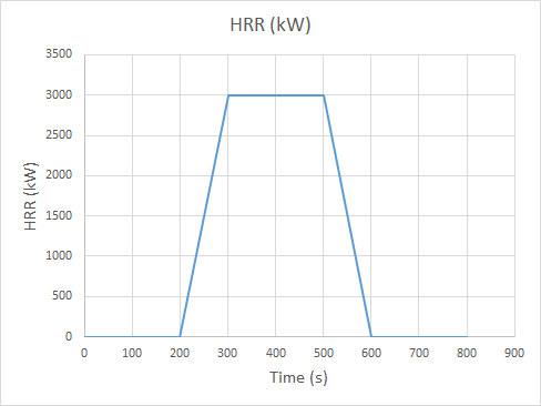
For this example, we used a very sooty fire that represents burning of Polyurethane GM27. The soot yield is 0.198 which results in a large amount of smoke. The fire has a surface area of 6 m² with a peak Heat Release Rate per Unit Area of 500 kW/m², giving a peak Heat Release Rate (HRR) of 3000 kW. The 3000 kW value was chosen based on the paper by Jones et al. (Jones, Noonan, and Riordan 2007). A simple ramp up to peak HRR and ramp down was used. This time history was selected to speed the calculation.

plot graph jet car park hrr input — Figure 24. Specified HRR of fire.

4.1.2. Results for First Design

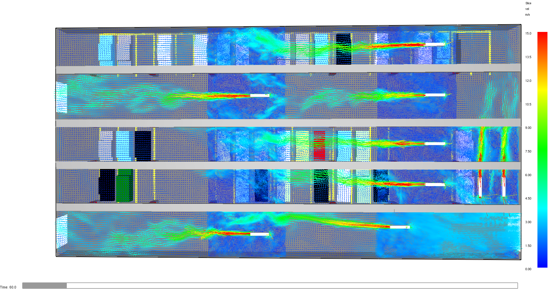
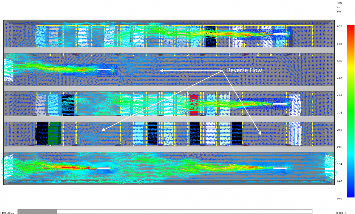
We will first look at the initial flow patterns before the fire starts. Figure 25 shows the corresponding flow vectors for the fast fan (18 m/s) case. In both cases, the primary flow is towards the exhaust exits, but there is some reverse flow in the lanes between the fans. The contours are shown just below the fans which are centered at Z = 2.75 m (the ceiling is at 3 m and the lower edge of the beams is at Z = 2.5 m). Finding a fan configuration with no reverse flow is not simple and requires design calculations.

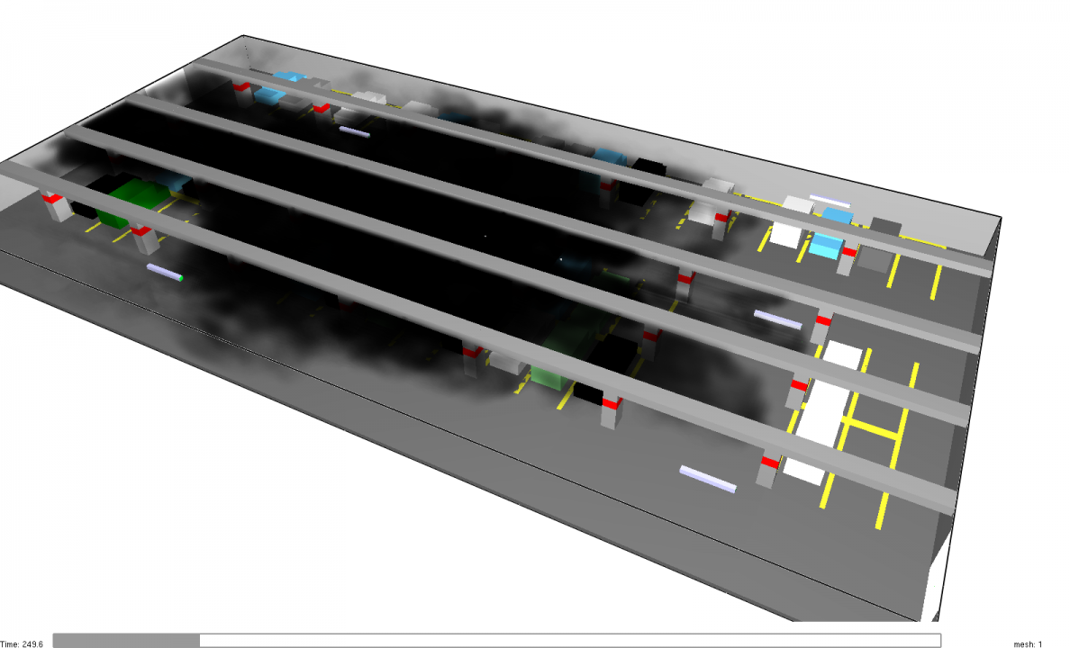
results jet car park flow vectors — Figure 25. Flow vectors at Z=2.5 m at 200 seconds.

The fire starts at 200 s, reaches a peak at 300 s, stays at the peak to 500 s, then ends at 600 s. At 250 s, when the Polyurethane GM27 fire has only reached half its peak value, the smoke already extends throughout much of the car park, as shown below. Figure 26 does show that the flow due to the jet fans tends to push the smoke to the exit. However, by 500 s, smoke completely fills the car park for both cases.

results scrn jet car park 250s — Figure 26. Smoke at 250 seconds.

At 500 s, the time of peak fire, smoke completely fills the car park.

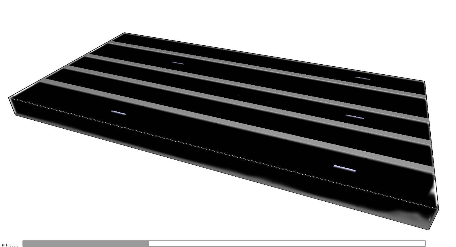
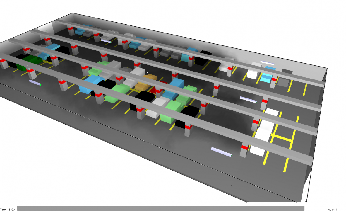
results scrn jet car park 500s — Figure 27. Smoke at 500 seconds.

After the fire stops, the jet fan flow begins to clear the air. At 1600 s, the fast fan case shows nearly complete clearing of the smoke.

results scrn jet car park 1600s — Figure 28. Smoke at 1600 seconds.

Heating of the air due to the fire has a large impact on the evacuation of smoke. Obviously, the heated air rises and then spreads when it contacts the ceiling.

But in addition, the heating of the air causes it to expand with two consequences:

Less fresh air flows into the car park
Although air velocity at the jet fan exits remains the same, the reduced density of the air means that the fans have less thrust to move the air.

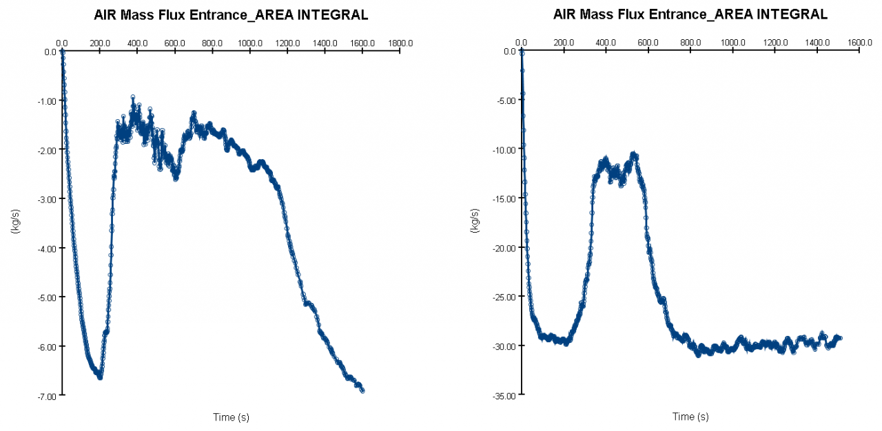
This effect can be seen in Figure 29, the plots of the entry air mass flux. Here we show both a slow and fast fan case. In both cases, when the fire starts, the fresh air flow into the model is reduced significantly. As the hot air is exhausted the fresh air flow again increases.

plot graph jet car park mass flow — Figure 29. Mass flow rate of supply air into car park. Image on left is for jet fan velocity of 4.5 m/s and image on right for jet fan velocity of 18 m/s.

4.1.3. Summary of First Design Results

The first design was not developed with any design calculations, it was just a guess that used the same jet fan parameters as used for the convergence study. The results show that the first design was not adequate:

The design has locations with reverse air flow.
After the fire starts, the high velocity of the hot air and smoke was able to overcome the air velocity due to the jet fans.
For this first design, the smoke spreads throughout the car park.
The change in air density due to heating reduced the efficiency of the fans (volume flow the same, mass flow and thrust reduced) and significantly reduced the amount of fresh air flowing into the car park.

Because of the poor performance of the first design, a re-design was required.

4.1.4. Second Design

An improved ventilation design was developed by James Allen at Fläkt Woods Group (james.allen@flaktwoods.com) and is shown in Figure 30.

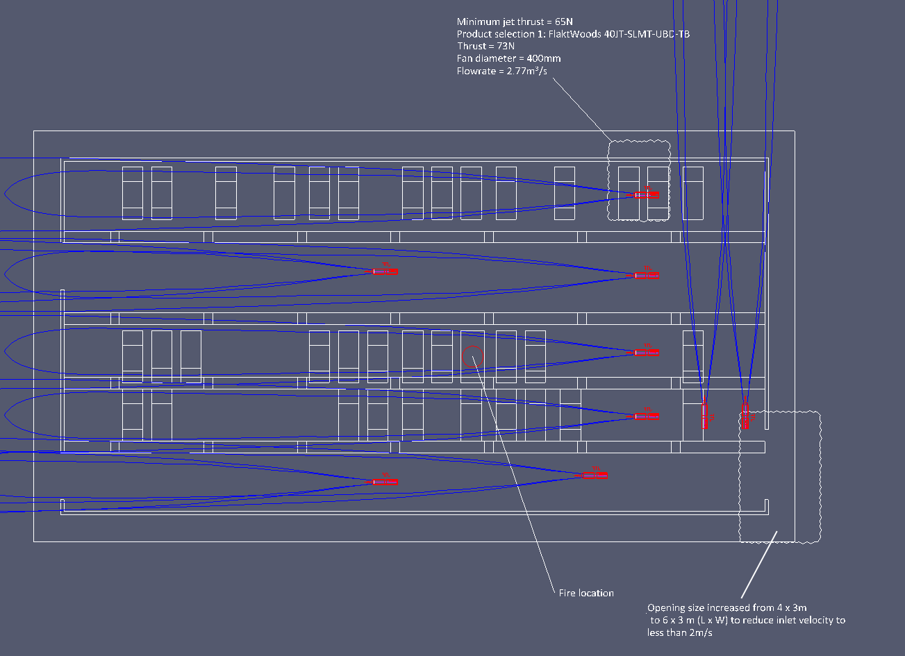
doc scrn jet fan redesign — Figure 30. Improved design of car park ventilation (James Wood)

Changes to the original design include:

Use of more powerful fans with a minimum thrust of 65 N. The recommended fan had a thrust of 73 N with a diameter of 400 mm and a flow rate of 2.77 m³/s.
Use 9 fans.
Rearrange the fans to enhance flow from the entry and a line of fans that moves air uniformly toward the exits.
Increase the area of the open supply from 4 m x 3 m to 6 m x 3 m, to reduce inlet flow to less than 2 m/s.

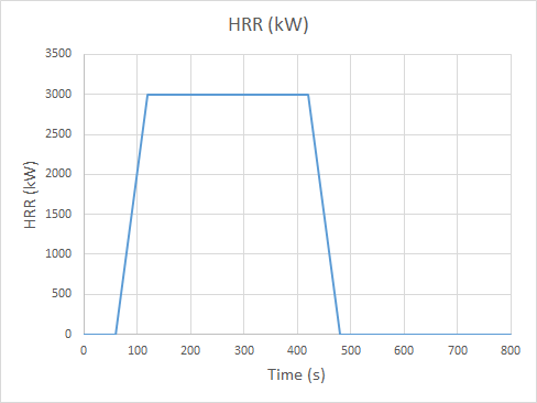
Although not a design change, because of the higher flow, the HRR time history was shortened, so that the ramp to full HRR occured from 60 s to 120 s. The fire then remained constant for 300 s to ensure that a steady state condition was met with respect to smoke, it then ramped down from 420 s to 480 s.

plot graph jet redesign hrr — Figure 31. Specified HRR of fire for new design calculation.

4.1.5. Validation Run for New Fan

Because the new design uses different fans, it was necessary to verify that the calculation gives acceptable results. The new fans have a diameter of 0.4 m. Using the 0.125 m mesh size, the representation of the fan is a 0.375 m x 0.375 m square. This gives a different area than the circular fan.

The thrust of a jet fan is given by:

Jet Thrust Equation

\[T_g=Q_dV_d\rho\]

Where:

\(T_{g}\) is the gross thrust.
\(Q_{d}\) is the volume flow of air at discharge.
\(V_{d}\) is the discharge velocity.
\(\rho\) is the air density.

To maintain the same theoretical thrust with a different area, the equivalent discharge velocity is 20.7 m/s and the flow rate is 2.9 m³/s. The results for a 0.375 m x 0.375 m jet fan with these equivalent conditions are shown below. In both cases the total jet fan length was 2.5 m. The velocity patch model used a 0.5 m short shroud and the HVAC model included a 0.375 m length downstream shroud. For both models, the centerline velocity decay and flow entrainment are less than the experimental correlations. Ideally, the mesh would be refined, but to keep reasonable run times, the assumed mesh dimensions will be used. Although the jet fan model with a velocity patch performs slightly better, it was decided to focus on the HVAC model because of its reliability. Using the HVAC model will provide conservative results with respect to the car park simulation, since it will be a lower flow entrainment corresponds to a longer time to clear the smoke.

plot graph jet redesign convergence results — Figure 32. Centerline velocity and flow entrainment for the 73 N thrust fan.

4.1.6. Results for Second Design

We first look at velocity vectors just before the fire starts. Compared to the first design, the flow velocities are more than twice as large. There are some locations of circulation, but most of the flow is towards the exits.

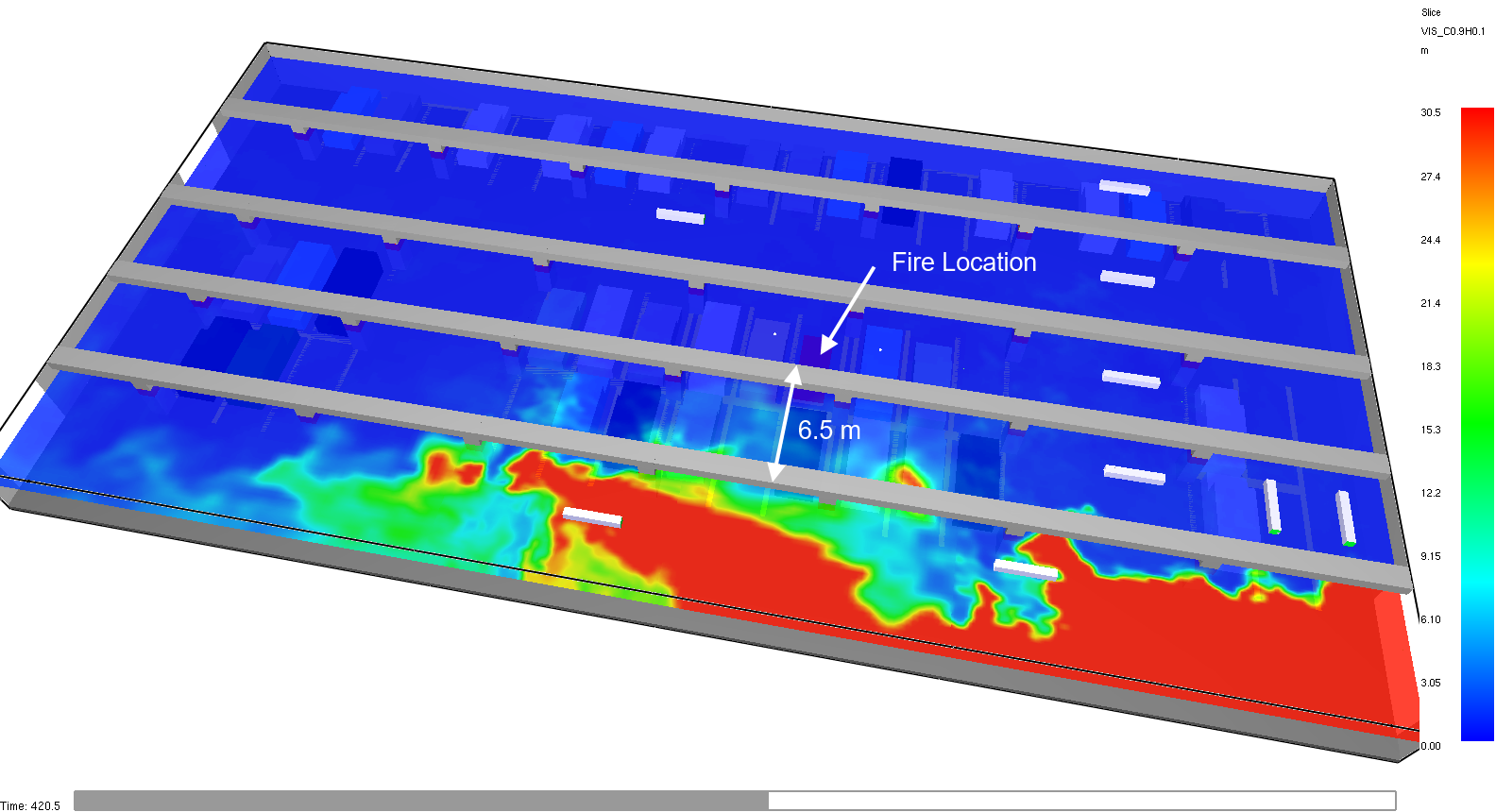
results scrn jet redesign hvac — Figure 33. Velocity vectors at 60 s, Z=2.5 m.

The visibility contours under full fire conditions are shown in Figure 34. This image shows that about 6.5 m from the fire, the visibility has increased to about 9 m.

results scrn jet redesign visibility — Figure 34. Visibility contours at 420 s, Z=2.0 m. These contours show visibility under full fire conditions. Red corresponds to greatest visibility.

The contours of temperature at 420 s and Z = 2.5 m are shown in Figure 35. The distance from the fire to a location where the temperature is less than 60 C is about 2 m. Because the fans operate in relatively cool air, the efficiency of the fans does not significantly change and the replacement entrance air flow was approximately constant at 52 m³/s.

results scrn jet redesign temperature — Figure 35. Temperature contours at 420 s, Z = 2.0 m. These contours show temperatures under full fire conditions.

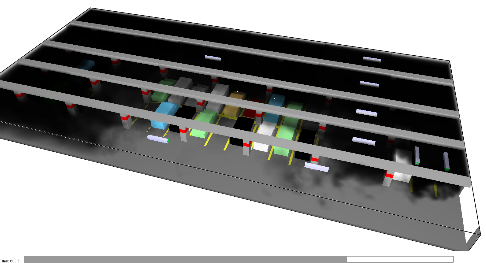
The smoke visualization at 420 s (peak fire) and 600 s (120 after end of fire) are shown in Figure 36 and Figure 37. By 800 seconds, the car park is cleared of smoke.

results scrn jet redesign smoke 420s — Figure 36. Smoke visualization at 420 s. This shows smoke under full fire conditions.

results scrn jet redesign smoke 600s — Figure 37. Smoke visualization at 600 s. This shows smoke 120 s after the end of the fire. Smoke is beginning to clear.

4.1.7. Summary of Re-Design Results

The re-design provided by James Allen at Fläkt Woods Group was satisfactory, meeting both visibility and temperature criteria.

4.2. Summary

This section has demonstrated an approach to simulating fire and smoke in a car park using FDS and PyroSim. The first (naive) design was not satisfactory, but a re-design proposed based on calculations met design criteria. This highlights the requirement that design calculations be understood and implemented when developing the smoke control system for a car park fire.

It is anticipated that the results are conservative for two reasons:

The selected jet fan model (HVAC duct with downstream shroud) under-estimates flow entrainment downstream of the fan.
The fire used for the simulation was very sooty, so this would under-estimate visibility.

5. Bibliograhpy

Awbi, H.B. 2003. Ventilation of Buildings. https://doi.org/10.4324/9780203476307.

Baturin, V. V. 1972. Fundamentals of Industrial Ventilation, by V. V. Baturin. Book. 3D, enl. ed. Translated by O. M. Blunn. Pergamon Press Oxford, New York.

Eck, Bruno. 2007. “Technische Strömungsmechanik.” https://doi.org/https://doi.org/10.1007/978-3-662-00793-8.

Jones, J.C., T. Noonan, and M.C. Riordan. 2007. “An Examination of Vehicle Fires According to Scaling Rules.” International Journal on Engineering Performance-Based Fire Codes 9 (3): 111–17.

Lu, S., Y.H. Wang, R.F. Zhang, and H.P. Zhang. 2011. “Numerical Study on Impulse Ventilation for Smoke Control in an Underground Car Park.” Procedia Engineering 11: 369–78. https://doi.org/https://doi.org/10.1016/j.proeng.2011.04.671.

McGrattan, et al., Kevin. 2020. Fire Dynamics Simulator Verification Guide Volume 2. Sixth Edition. National Institute of Standards and Technology, Gaithersburg, Maryland, USA: NIST.

Ricou, F. P., and D. B. Spalding. 1961. “Measurements of Entrainment by Axisymmetrical Turbulent Jets.” Journal of Fluid Mechanics 11 (1): 21–32. https://doi.org/10.1017/S0022112061000834.

v.d.Giesen, B.J.M., S.H.A. Penders, M.G.L.C. Loomans, P.G.S. Rutten, and J.L.M. Hensen. 2011. “Modelling and Simulation of a Jet Fan for Controlled Air Flow in Large Enclosures.” Environmental Modelling & Software 26 (2): 191–200. https://doi.org/https://doi.org/10.1016/j.envsoft.2010.07.008.

Viegas, João Carlos. 2010. “The Use of Impulse Ventilation for Smoke Control in Underground Car Parks.” Tunnelling and Underground Space Technology 25 (1): 42–53. https://doi.org/https://doi.org/10.1016/j.tust.2009.08.003.

To download the most recent version of PyroSim, please visit the PyroSim page and click the button for the current release. If you have any questions, please contact support@thunderheadeng.com

Modeling Jet Fans

Related Tutorials