To follow along with this tutorial, download the relevant files here.
Introduction
FDS assumes one-dimensional heat conduction into the surfaces of solid obstructions. With proper modeling, you can couple the front and back face temperatures of an obstruction so that heat flows through the obstruction. This post demonstrates heat transfer through obstructions, including radiative and convective fluxes on the surface.
One-dimensional Heat Conduction
A common point of confusion when discussing heat conduction in FDS is that FDS only performs a transient, one-dimensional calculation of heat transfer. For most fire simulation situations, this is a computationally fast and appropriate approximation of real heat conduction. For example, the surface temperature of a hollow wall constructed of gypsum board is well represented by transient, one-dimensional heat conduction through the gypsum board with an assumed air gap boundary condition on the back of the gypsum board.
The one-dimensional assumption does introduce limits. For example, local heating of an obstruction will not spread radially and heating one side of an obstruction will not heat adjacent sides. In addition, there are constraints on the geometry of the obstruction when calculating heat transfer through an obstruction.
Heat Conduction in an Obstruction
In FDS, an obstruction is a three-dimensional solid object that blocks flow. Often, obstructions represent the walls, floor, and ceiling of a model, but they can be any object such as a sofa or a car. In this post, we will focus on heat conduction in an obstruction that has solid surfaces. We will not include pyrolysis of the solid.
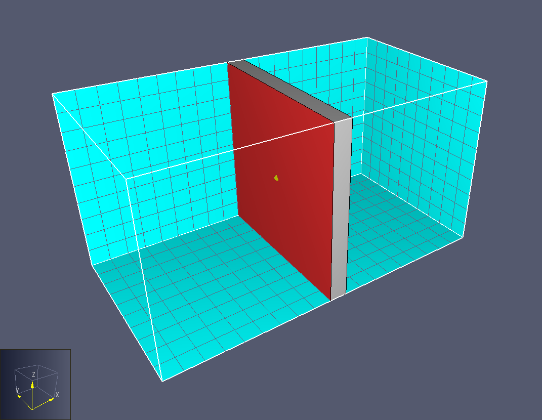
The simplified model we will use is shown in Figure 1.
The obstruction is rectilinear and one 0.1 m cell thick, with six solid heat conducting surfaces that are defined using materials..
The red face is heated by an external radiative flux, the other five gray surfaces are not heated.
All boundaries of the model are OPEN to an ambient temperature of 20 ºC.
The mesh extends 1.9 m in the X direction, and 1.0 m in the Y and Z.
The mesh cell size is a uniform 0.1 m.
An obstruction is created in steps: first we define materials, next we use the materials to create surfaces, finally we use the surfaces as part of the obstruction. We describe each of these steps and the available options in the following sections.
Material Input
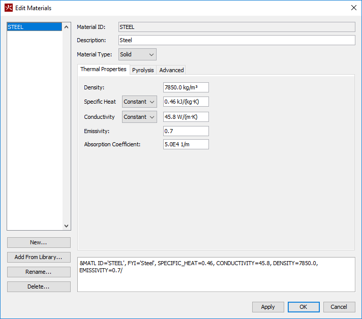
A material defines the standard heat conduction properties: density \(\rho\), specific heat \(c\), and conductivity \(k\).
It also includes the material emissivity, which is used when calculating radiative heat flux from the surface, and the absorption coefficient, which defines the depth that radiation penetrates to deposit energy.
The default emissivity is 0.9 and the default value of the absorption coefficient is 5.0E4 1/m.
The default absorption coefficient deposits all radiation energy at the boundary surface, with no penetration.
Figure 2 shows the PyroSim Edit Materials dialog with values that define steel.
Surface Input
Heat conduction options are defined in the surface. In this example, we will only discuss a solid surface that conducts heat (a layered surface), but there are simpler temperature boundary condition options, such as ADIABATIC, available in FDS. See an earlier post Radiation and Convection on Surfaces for a discussion of these options.
For a conducting solid, the surface geometry is defined by layers of materials with specified thicknesses.
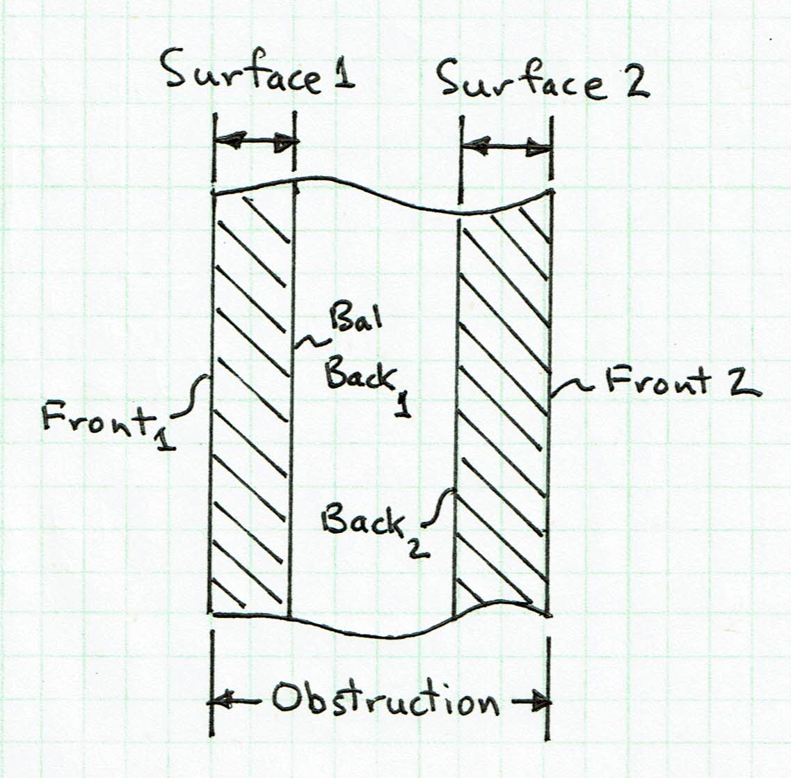
This raises a second common point of confusion related to heat conduciton - the thickness used for the surface heat conduction calculation is independent of the thickness of the obstruction using that surface.
This is illustrated in Figure 3, where the obstruction thickness could be 0.1 m, but the surface thickness used for the heat transfer calculation could be 0.02 m, as in our example.
Recall also that all geometry in FDS snaps to the mesh coordinates, an obstruction that is 0.08 m thick in a mesh with 0.1 m cell size, will snap to be 0.1 m thick.
The front of a conducting surface is heated by radiation and convection. The convective heat flux is given by:
where \(h\) is the convective heat transfer coefficient, \(T_{g}\) is the gas temperature, and \(T_{w}\) is the surface wall temperature.
In general, the radiative heat flux is a function of radiation intensity and geometry. For the special case where the radiation shape factor is unity, the radiative heat flux is given by:
where \(\epsilon\) is the emissivity, \(\sigma\) is the Stefan-Boltzmann constant (\(5.670 \times 10^{-8} \: W \cdot m^{-2} \cdot K^4\)), \(T_{w}\) is the wall temperature, and \(T_{a}\) is the ambient temperature surrounding the surface.
For steady state heat conduction through a uniform material with no internal heat generation, the conductive heat flux is given by:
where \(k\) is the conductivity, \(thick\) is the thickness of the material, and \(T_{back}\) and \(T_{front}\) are the wall temperatures.
We will use equations 1, 2, and 3 to calculate an energy balance at the surface.
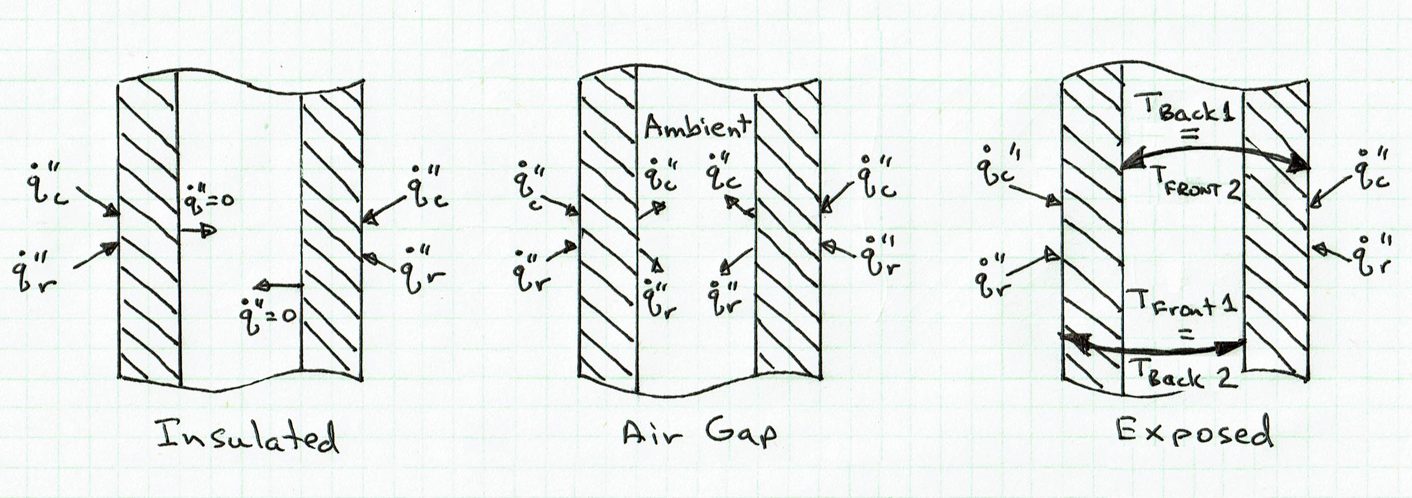
In FDS, the back side of the surface can have three boundary conditions, illustrated in Figure 4.
- The INSULATED option means that there is no heat loss from the back side of the material.
- The VOID (air gap) option assumes the wall is open to ambient conditions, with radiative and convective heat fluxes removing heat.
- The EXPOSED option couples the back of surface 1 to the front of surface 2. This means that heat can be conducted through the obstruction, so heating the front of surface 1 will result in raising the temperature of the front of surface 2. However, the EXPOSED option is only valid for obstructions that are less than or equal to one cell thick with a non-zero volume of computational domain on the other side of the obstruction. If the obstruction is on the boundary of the domain or if the obstruction is more than one cell thick (cases where the front of surface 2 is not exposed to gas), the boundary condition is changed to VOID and exposed to an air gap at ambient conditions.
Only the EXPOSED option can be used to calculated heat transfer through the obstruction. See the FDS User Guide section Back Side Boundary Conditions for further background.
The details of defining a solid conducting surface in the PyroSim interface are shown below.
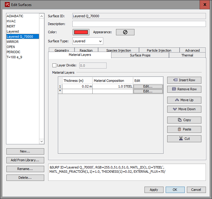
- Figure 5 shows the Material Layers tab of the Edit Surfaces dialog. The user inputs the thickness and the material composition of the layer. In general the composition can be a mixture, in this case only the STEEL material forms the layer.
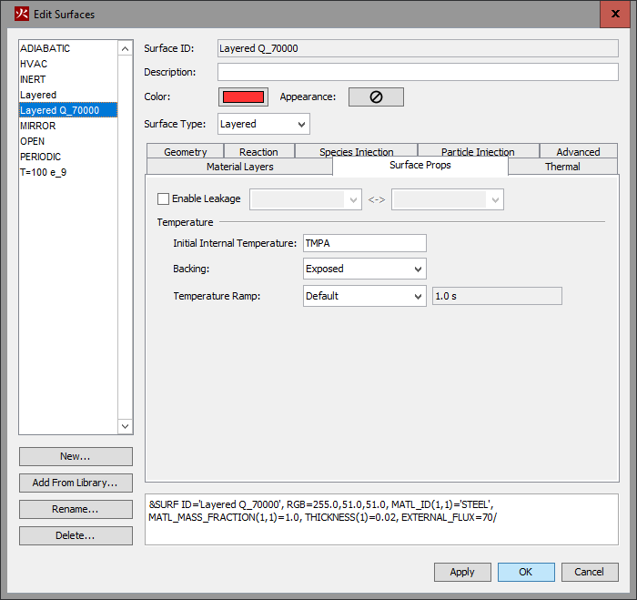
- Figure 6 shows the Surface Props tab where the back side boundary condition is selected. In this case, the option is EXPOSED.
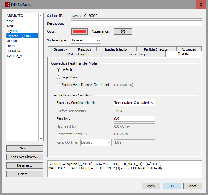
- The front side boundary options for surfaces are selected on the Thermal tab, Figure 7. For conducting solid surfaces, only the Temperature Calculated option is valid. Although the PyroSim interface implies that the surface emissivity can be specified, the material emissivity will be used for conducting solid surfaces. The PyroSim interface will be corrected in a future release.
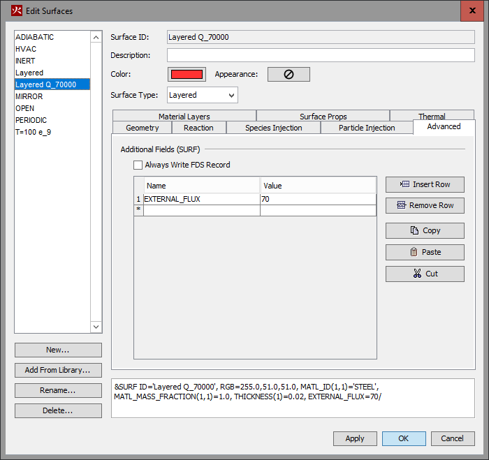
- Figure 8 shows how to specify an EXTERNAL_FLUX using the Advanced tab.
This option was only used for the heated surface of the obstruction.
The value is
70 kW/m2.
Obstruction Input
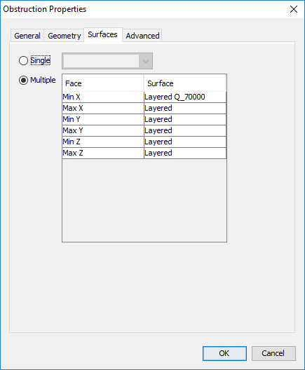
Each side of an obstruction can have a different surfaces. Figure 9 shows the surface definitions for our simple obstruction. Only the Min X side of the obstruction is heated.
Transient Solutions
To verify the transient heat conduction calculation we will use the transient, one-dimensional heat conduction into a semi-infinite solid. This solution will be valid during the initial transient while the back surface temperature remains at the initial temperature.
The solutions for transient heat flow in a semi-infinite solid can be found in any standard text. The transient temperature for a uniform initial temperature with the surface temperature suddenly raised to a fixed value is:
where \(T_{0}\) is boundary surface temperature and \(T_{i}\) the initial temperature.
If the surface is suddenly exposed to a constant heat flux, the solution is given by:
Heat Conduction Example
We have now completed the description of the model, so let us review the results.
We expect to see an initial transient followed by a long-term steady state response.
The initial transient results are shown in Figure 11, a plot through the thickness of the surface.
The analytic solution is calculated using the material properties in Figure 2 and a heat flux of 49 kW/m2 (equal to the EXTERNAL_FLUX value of 70 kW/m2 multiplied by the material emissivity of 0.7).
The FDS results were obtained using devices located uniformly at 0.001 m intervals through the depth of the surface.
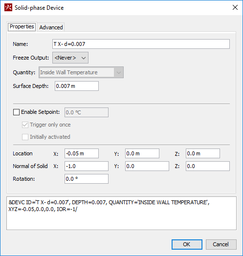
&DEVC ID='T X- d=0.007', DEPTH=0.007, QUANTITY='INSIDE WALL TEMPERATURE', XYZ=-0.05,0.0,0.0, IOR=-1/
At 2.06 s the transient has not reached the back side, so the solution is independent of the back side boundary condition and only one FDS result is presented.
FDS uses a one-dimensional numerical solution for the solid surface. The FDS result is not smooth because the Inside Wall Temperature device used to extract the FDS results does not interpolate between the numerically calculated node values. See the FDS User Guide section Solid Phase Numerical Gridding Issues and the FDS Technical Reference the section Solving the 1-D Heat Conduction Equation for more information on options to control the numerical solution. The FDS solution in this example used the default options, with larger node spacing in the center of the surface and smaller spacing near both surfaces.
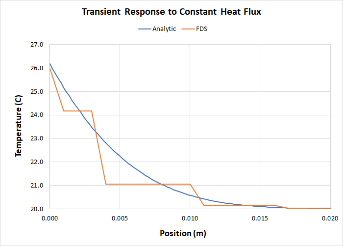
As shown by the front temperatures (Analytic = 26.17 ºC, FDS = 25.96 ºC) and back temperatures, the FDS solution matches the analytic solution.
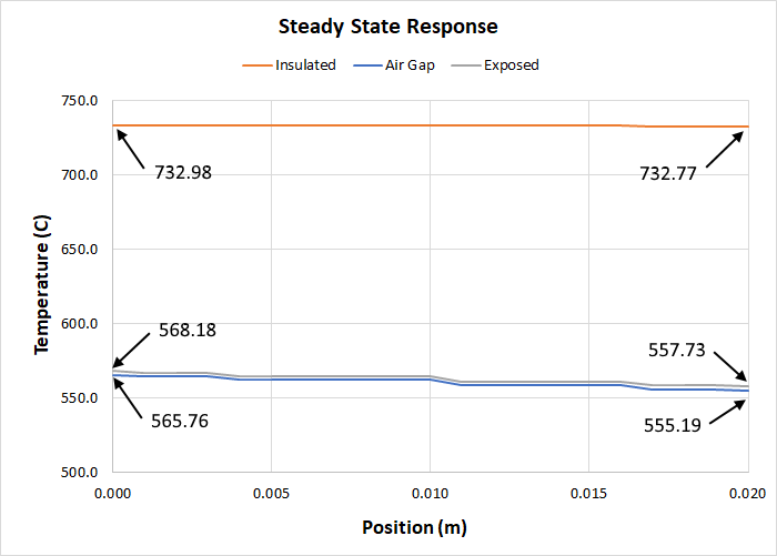
The near steady state solutions at 2500 s are shown in Figure 12.
The INSULATED boundary condition has reached a nearly uniform temperature.
The VOID (air gap) solution and the EXPOSED solution show a temperature gradient between the front and back faces.
The air gap solution is slightly lower, since the convective heat loss is to the constant ambient temperature rather than the calculated back gas temperature.
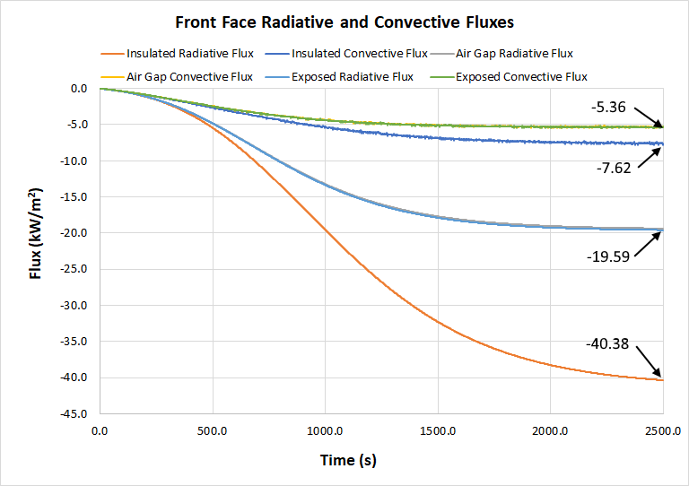
The radiative and convective fluxes for the front face are shown in Figure 13.
The negative values indicate that heat is being removed from the surface.
The FDS device used to measure radiative flux at the front surface includes both the applied EXTERNAL_FLUX and the radiative flux from the surface to the environment.
Figure 13 shows only the radiative flux from the surface, which was obtained by subtracting 49 kW/m2 (the EXTERNAL_FLUX times emissivity) from the FDS device output.
Because the results for VOID (air gap) and EXPOSED boundary conditions are similar, numerical values given at 2500 s are those for the EXPOSED case.
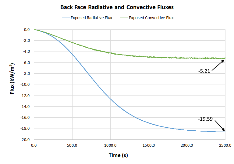
Fluxes for the back face are given in Figure 14. The data for the INSULATED and VOID (air gap) boundary conditions cannot be output by devices, so the graph only shows results for the EXPOSED boundary condition.
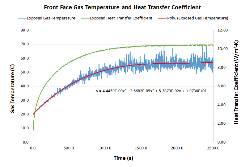
The values of hot gas temperature and heat transfer coefficient for the front face of the EXPOSED case are shown in Figure 15. These values are used to calculate the convective flux from the surface. The heat transfer coefficient is relatively smooth, but the hot gas temperature fluctuates. The cubic polynomial gives a smoothed result for temperature.
Remember that heat transfer through the obstruction is only calculated for the EXPOSED surface.
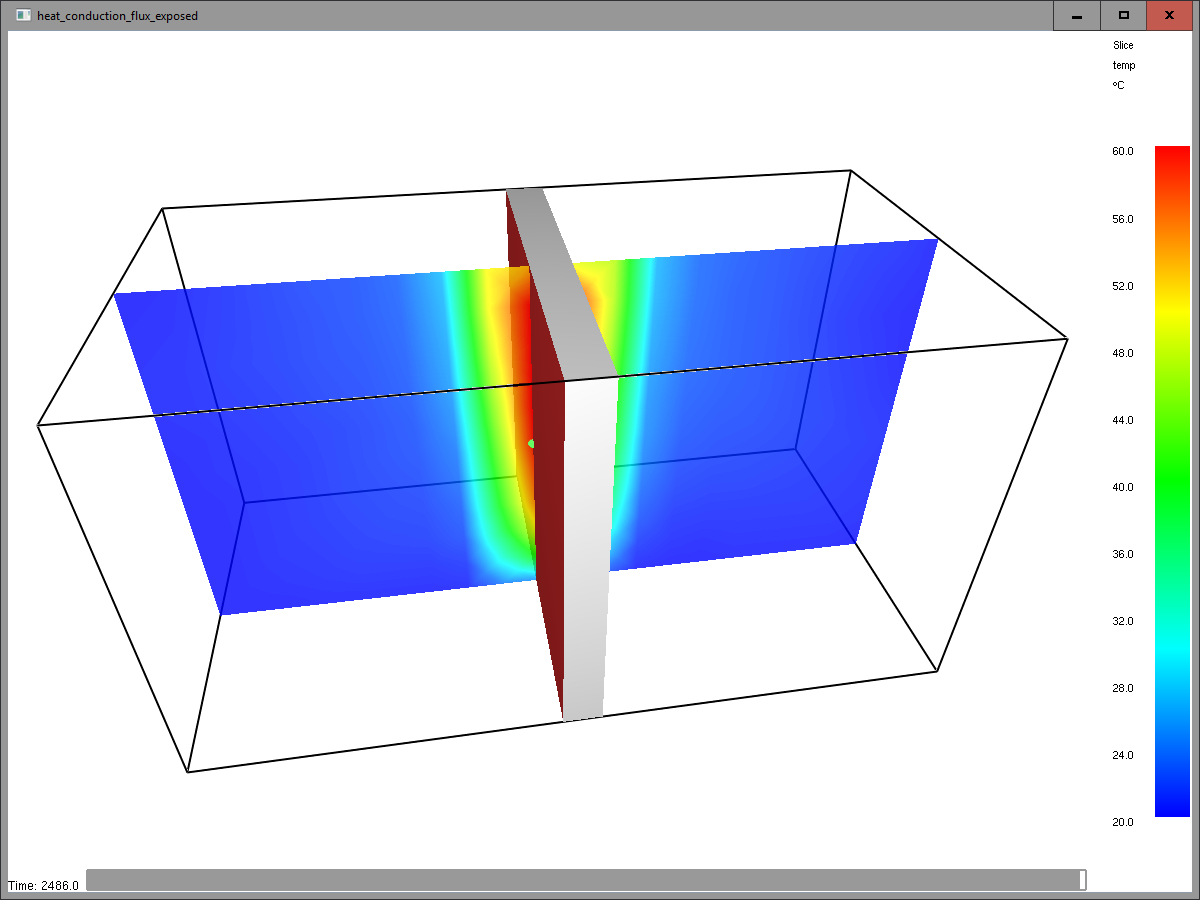
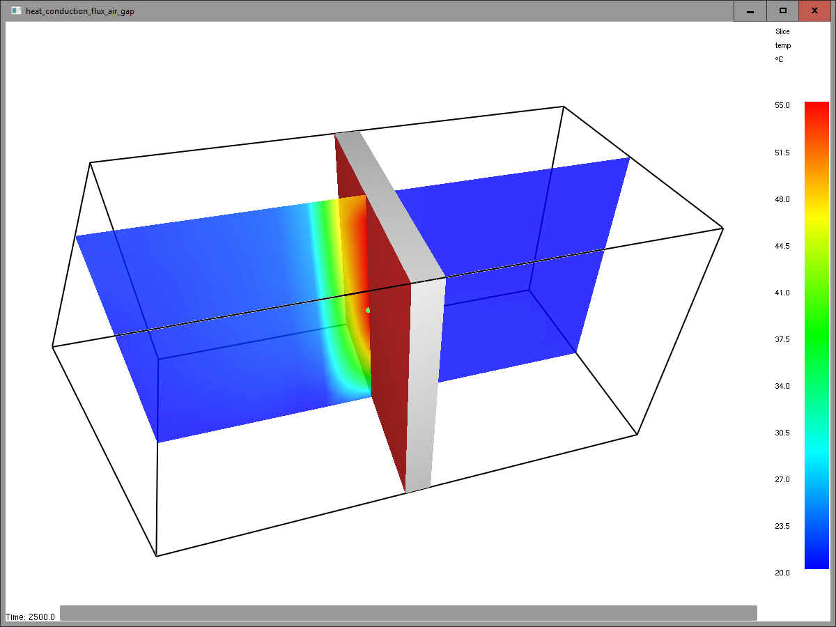
This is illustrated in Figure 16 and Figure 17, which shows air temperature contours at 2500 s.
For all cases, we heat the Min X face of the obstruction.
The EXPOSED case results in heat transfer through the obstruction and the air on the Max X face side is heated.
For the AIR GAP case, there is no heat transfer through the obstruction and the air on the Max X face is not heated.
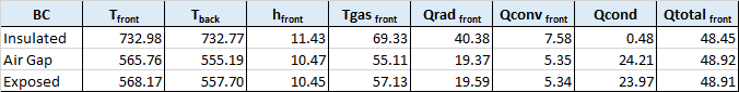
Heat Flux Balance
We can independently calculate the heat flux balance at the surface using Convective Heat Flux Equation, Radiation Heat Flux Equation if Radiation Shape Factor is 1.0, and Steady-State Conductive Heat Fluc Through a Uniform Material with no Internal Heat Generation.
The results of this calculation are shown in Figure 13 for the front surface at 2500 seconds.
These can be compared to the FDS results previously given on Figure 18.
The values are the heat fluxes leaving the front surface, so the total of the three fluxes matches the input heat flux of 49 kW/m2.
Summary
We have demonstrated the different heat conduction options for a solid surface in FDS. FDS only performs a one-dimensional calculation. The back face options include INSULATED, VOID (air gap), and EXPOSED. The EXPOSED option couples the temperatures of the opposite sides of the obstruction, which simulates heat conduction through the obstruction.
The transient response was verified in Figure 18 using the transient response of a semi-infinite solid to a constant surface flux. The steady state fluxes were verified by calculating the convective, radiative, and conductive fluxes based on the FDS surface temperatures, heat transfer coefficient, and hot gas temperature. The total flux was in equilibrium with the input eternal flux.
When using the EXPOSED option, the user must remember that it is only valid for obstructions that are less than or equal to one cell thick with a non-zero volume of computational domain on the other side of the obstruction.
To download the most recent version of PyroSim, please visit the the PyroSim Support page and click the link for the current release. If you have any questions, please contact support@thunderheadeng.com
Related Tutorials
Tutorial demonstrating how to model Radiation and Convection on Surfaces in Pyrosim.
(Legacy) Tutorial to experience the fundamental features of PyroSim
Tutorial demonstrating how to use PyroSim/FDS to Maximize Solar Panel Convective Cooling.
Tutorial to experience the fundamental features of Pathfinder
Tutorial demonstrating how to verify HVAC Pressure Drop in Pyrosim.
Tutorial demonstrating how to model a fire in Pyrosim.
How to simplify post-processing data collection with seasonal scenarios and scheduled stairwell temperatures.
Video tutorial demonstrating how to avoid creating unwanted gaps in the geometry of a Pathfinder model.