 |  |
General usage information for Ventus
Thunderhead Engineering makes no warranty, expressed or implied, to users of Ventus, and accepts no responsibility for its use. Users of Ventus assume sole responsibility under Federal law for determining the appropriateness of its use in any particular application, for any conclusions drawn from the results of its use, and for any actions taken or not taken as a result of analyses performed using these tools.
Users are warned that Ventus is intended for use only by those competent in the fields of fluid dynamics, thermodynamics, combustion, and heat transfer, and is intended only to supplement the informed judgment of the qualified user.
The software package is a computer model that may or may not have predictive capability when applied to a specific set of factual circumstances. Lack of accurate predictions by the model could lead to erroneous conclusions with regard to fire safety. All results should be evaluated by an informed user.
All other product or company names that are mentioned in this publication are tradenames, trademarks, or registered trademarks of their respective owners.
Throughout this document, the mention of computer hardware or commercial software does not constitute endorsement by Thunderhead Engineering, nor does it indicate that the products are necessarily those best suited for the intended purpose.
We would like to thank Steven Emmerich, William Stuart Dols, Brian Polidoro, and Andrew Persily in the Indoor Air Quality and Ventilation Group at the National Institute of Standards and Technology. They are the primary authors of CONTAM and associated programs, without which Ventus would not exist. They have been gracious in their responses to our many questions.
We would also like to gratefully acknowledge engineers at Performance Based Fire Protection Engineering, Coffman Engineers, Inc., and Jensen Hughes for their guidance and feedback on early versions of Ventus.
Any opinions, findings, and conclusions or recommendations expressed in this material are those of the authors and do not necessarily reflect the views of the external contributors.
Ventus is a graphical user interface for CONTAM version 3.4.0.6. CONTAM is closely integrated into Ventus, and is developed at the National Institute of Standards and Technology (NIST).
Below is an overview of CONTAM from the NIST website:
CONTAM is a multizone indoor air quality and ventilation analysis computer program developed to help you determine:
- airflows: infiltration, exfiltration, and room-to-room airflows in building systems driven by mechanical means, wind pressures acting on the exterior of the building, and buoyancy effects induced by the indoor and outdoor air temperature difference.
- contaminant concentrations: the dispersal of airborne contaminants transported by these airflows; transformed by a variety of processes including chemical and radio-chemical transformation, adsorption and desorption to building materials, filtration, and deposition to building surfaces, etc.; and generated by a variety of source mechanisms, and/or
- personal exposure: the prediction of exposure of occupants to airborne contaminants.
CONTAM can be useful in a variety of applications. Its ability to calculate building airflow rates and relative pressures between zones of the building is useful for assessing the adequacy of ventilation rates in a building, for determining the variation in ventilation rates over time, for determining the distribution of ventilation air within a building, and for estimating the impact of envelope air-tightening efforts on infiltration rates and associated energy implications. CONTAM can has been dynamically coupled with energy analysis programs including EnergyPlus and TRNSYS. The program has been used extensively for the design and analysis of smoke management systems. The prediction of contaminant concentrations can be used to determine the indoor air quality performance of buildings before they are constructed and occupied, to investigate the impacts of various design decisions related to ventilation systems and building material selection, to evaluate indoor air quality control technologies, and to assess the indoor air quality performance of existing buildings. Predicted contaminant concentrations can also be used to estimate personal exposure based on occupancy patterns within a building model.
Additionally,
It is important to note that CONTAM provides a macroscopic model of a building. In this macroscopic view, CONTAM considers Zones as well-mixed. CONTAM characterizes well-mixed Zones using a discrete set of state variables, such as temperature, pressure, and contaminant concentrations. Temperature and contaminant concentration do not vary spatially within a Zone, and contaminants mix instantly throughout Zones. However, pressure does vary hydrostatically within all Zones. (Dols and Polidoro 2020)
Over time, Ventus will support more of the capabilities of the ContamX program. The multi-zone lumped-parameter approach enables fast solutions compared to a more rigorous CFD model such as PyroSim.
The Ventus interface provides immediate input feedback and ensures the correct format for the CONTAM input file.
In summary, Ventus helps you quickly and reliably build complex pressurization, ventilation, and contaminant transport models.
In preparing this manual, we have liberally used descriptions from the CONTAM User Guide (Dols and Polidoro 2020). A link to the CONTAM User Guide is included in Ventus on the Help menu. You can also download documentation, executables, and verification and validation examples from the CONTAM webpage.
The following is a full list of changes made in this version of Ventus.
+ symbol.See the following sections for known issues with this release of Ventus.
The field value Minimum OA Flow in the Edit Air Handling System (AHS) dialog is overwritten in ContamX simulations. A mass flow equal to 100% of flow into the Supply of the AHS is implied; 0 kg/s (lbm/s) is recirculated for all AHS.
Ventus does not allow recirculation of air with the AHS utility.
As described in the CONTAM User Guide, an implicit f0=1.0 will override the Minimum OA Flow value.
A user may enter a small value as the Minimum OA Flow, intending to reduce the amount of Outdoor air and create recirculation.
There is 100 scfm airflow into the Supply of AHS SimpleAHS01.
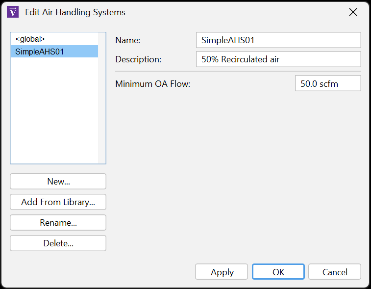
The user enters 50 scfm with the intention of modeling an exchange resulting in 50% outdoor air into the Supply, or 50% recirculation.
Despite the values in Figure 1, 100 scfm of air sent into the supply is outdoor air (100% OA, 0% Recirculation).
To work around this issue, assume that 100% of the airflow into any AHS Supply is from the Ambient Zone.
Do not use the Minimum OA Flow field.
The Leakage Area tab on the Flow Path Properties Panel presents two fields that are not helpful for non-Powerlaw Model Flow Elements.
Q vs P Flow ElementSelf-regulating Vent Flow ElementConstant Mass Flow Fan, Constant Volume Flow Fan, and Performance Curve Flow ElementsTwo-way - One Opening and Two-way - Two Opening Flow Elements
In the worst-case scenario, a user may enter a value into the Items field. The value would be represented in the UI, and would impact the Flow Path computation.
To resolve this issue, for impacted Flow Elements, users should NOT select the Items field in Leakage Area and should NOT enter a value in the Items field.
There is an effort underway to rename the Leakage Area tab and restructure the Area, Length and Items multiplier fields on the Properties Panel.
| Intel | AMD | |
| Operating System: | Windows 10 | Windows 10 |
| Processor: | Core i5 3570 (4 core) | Athlon x4 970 (4 core) |
| Graphics Card: | Integrated HD Graphics | Integrated HD Graphics |
| Memory: | 8GB RAM | 8GB RAM |
| Intel | AMD | |
| Operating System: | Windows 11 | Windows 11 |
| Processor: | Core i7 8700 (6 Cores / 12 Threads) | Ryzen 7 1700 (8 Cores / 12 Threads) |
| Graphics Card: | NVIDIA GeForce GTX570 / AMD Radeon HD7870 | NVIDIA GeForce GTX570 / AMD Radeon HD7870 |
| Memory: | 16GB RAM | 16GB RAM |
When installing Ventus, the installer will either upgrade and existing version of the software, or install Ventus if it has not been previously installed. Installation requires Administrator privileges as the installer adds processes to the operating system for license management and ContamX simulation. The installer will also add Windows Defender exclusions for the bundles ContamX executables in order to avoid performance issues.
Ventus will regularly check for and notify the user of available updates to the software when configured to do so. By default, Ventus will check for updates on startup and display the relevant information in the Check For Updates dialog when one is available.
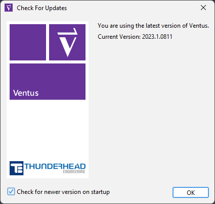
Users can also access this dialog by navigating to Help › Check For Updates.
The dialog can be disabled on startup by unchecking Check for newer version on startup. Users can skip the current update by clicking the Skip Update button, preventing update notifications until a new version is released beyond the latest version.
The latest version of Ventus can be downloaded on the Ventus Download Page.
You can view pricing, purchase licenses, or request a free trial via the Ventus Pricing Page. Ventus trials are full-featured trials, meaning there is no functional difference between a trial license and fully licensed version of Ventus.
See the Ventus Fundamentals course where we provide a series of modules that guide you through increasingly complex modeling concepts.
Ventus provides two primary panels for working on Ventus models, the Object Tree and the 2D/3D Workspace. If an object is added, removed, or selected in one panel, the other will simultaneously reflect the change. Each panel is briefly described below.
The Object Tree helps you quickly find objects and data that are not always easily accessible from the Workspace.
The Object Tree is arranged in the following groups:
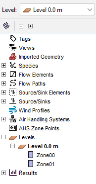
The buttons directly above the Object Tree performs the following actions:
The Level selection box above the Object Tree (see the top of Figure 4) can be used to manage levels. Any time a Zone is created it is added to a level group matching the current selection in the Level box. Changing the selection in the Level box will cause the newly selected level to be shown and all other levels to be hidden. Also, the Z property for all drawing tools will automatically default to the height of the level currently selected in the Level box. The visibility of any object or group of objects can always be manually set using the right-click context menu. This technique is useful if you want to show two levels at the same time (e.g. when creating a stairwell shaft).
There are additional options available to manage level view and selection in the Level Creation panel (Figure 15), which is detailed in Automatically Creating Levels. This panel is available when nothing is selected and no tools are active.
The Show lower level option in the Active Level section, when selected, will always show the level immediately below the current active level. This is to help with drawing snap references and to check alignment of zones and components in the model. If unselected, the level immediately below the active level will be hidden.
If Show lower level is selected, then an additional option will be available to Limit selection to active level. This will limit selection to only items that belong to the current active level.
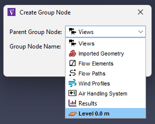
Groups can be used to hierarchically organize the model. Groups can only be seen in the Object Tree. Users can nest groups inside other groups, allowing the user to work with thousands of objects in an organized way. When the user performs an action on a group, that action will be propagated to all objects in the group.
To create a new group:
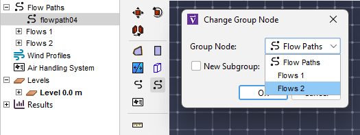
An object can be moved from one group to another at any time.
To change an object’s group:
The 2D/3D Workspace as shown in Figure 7 is the panel where much of the modeling work is performed in Ventus.
The Workspace contains tools to draw Zone geometry, Flow Paths, and AHS zone point locations.
There are two camera projection modes.
The main difference between the two modes is that the 3D mode allows the model to be viewed from any direction, whereas the 2D mode only allows viewing from one, orthographic direction.
In addition, the 3D mode contains no snap grid, whereas the 2D mode does.
The 3D mode is entered by selecting the perspective camera, ![]() , and the 2D mode is entered by selecting one of the orthographic cameras,
, and the 2D mode is entered by selecting one of the orthographic cameras, ![]() ,
, ![]() , or
, or ![]() .
.
Several buttons are located at the top of the Workspace, providing various camera modes, display options, and navigation modes. This is the static Navigation toolbar. The panel under this is known as the Properties Panel and is selection context-sensitive.
The panel of buttons on the left shows move/copy and drawing tools. The small panel at the bottom displays messages relevant to the current tool.
The Ventus global coordinate system has x-y-z axes in the lower left corner of the 2D/3D Workspace as shown in Figure 7. Wind directions are defined relative to the global coordinate system. North is aligned with the positive y-axis; East is aligned with the positive x-axis.
Several tools are provided for navigating through the model in the 3D mode including orbit, roam, pan, and zoom tools.
Ventus can be navigated while using the Select/Edit Objects tool, ![]() .
To Orbit the camera while in 3D mode, use a right-click and drag combination.
Similarly, use a middle-click and drag to Pan in perspective view.
To Zoom in and out of the model, use the scroll wheel on the mouse.
.
To Orbit the camera while in 3D mode, use a right-click and drag combination.
Similarly, use a middle-click and drag to Pan in perspective view.
To Zoom in and out of the model, use the scroll wheel on the mouse.
A navigation tool for the 3D mode is the Orbit tool, ![]() .
.
Another navigation tool in the Workspace is the Roam tool, ![]() .
This tool allows the camera to move in and out of the model at will.
It has a higher learning curve but is the most flexible viewing tool because it allows the camera to be placed anywhere in the model.
This tool can work in three different modes.
In the first two modes, the movement speed of the camera can be changed by holding CTRL and spinning the mouse wheel up or down.
Spin it up to increase the speed and down to decrease the speed.
.
This tool allows the camera to move in and out of the model at will.
It has a higher learning curve but is the most flexible viewing tool because it allows the camera to be placed anywhere in the model.
This tool can work in three different modes.
In the first two modes, the movement speed of the camera can be changed by holding CTRL and spinning the mouse wheel up or down.
Spin it up to increase the speed and down to decrease the speed.
This mode smoothly animates the camera to any location using only the mouse. To do so, press and release the middle mouse button. The cursor will disappear, and the tool will enter Mouse-only Mode. In this mode, moving the mouse will look around as in the other modes except that the mouse button doesn’t have to be pressed. Pressing and dragging the left mouse button will move the camera in the X-Y plane. The further the mouse is moved from its button press, the faster the camera will move. This can simulate the effect of accelerating the camera. Doing the same with the middle mouse button will cause the camera to move forward/backward in the X-Y plane with changes along the Y mouse axis and turn left/right with changes along the X mouse axis. Pressing and dragging the right mouse button will move the camera along the Z axis in the same manner. To exit Roam Mode, press and release the middle mouse button again or press ESC on the keyboard.
The other navigation tools include a Pan/Drag tool, which moves the camera left and right and up and down, a zoom tool, which zooms in and out of the model while click-dragging, and a zoom box tool, which allows a box to be drawn that specifies the zoom extents.
Navigation in the 2D projection is simpler than in 3D. The Selection/Manipulation tool not only allows objects to be selected if single-clicked, but it allows the view to be panned by middle or right-clicking and dragging, and the view to be zoomed by using the scroll wheel. The drag and zoom tools are also separated into separate tools for convenience.
At any time, the camera can be reset by pressing CTRL+R on the keyboard, or selecting Reset All ![]() .
This will cause the entire model to be visible in the current view.
For all navigation tools but the Roam tool, reset will make the camera look down the negative Z axis at the model.
For the roam tool, however, reset will make the camera look along the positive Y axis at the model.
.
This will cause the entire model to be visible in the current view.
For all navigation tools but the Roam tool, reset will make the camera look down the negative Z axis at the model.
For the roam tool, however, reset will make the camera look along the positive Y axis at the model.
The camera can also be reset to the current selection at any time by pressing CTRL+E. This will cause the camera to zoom in on the selected objects and the orbit tool to rotate about the center of their bounding sphere.
Very similar to resetting the camera, the view can be fit by pressing F on the keyboard or selecting the Fill View tool, ![]() .
The difference between the Fill View and Reset All tools is that filling the screen does not change the view angle of the camera.
Instead, the camera will recenter/zoom to fit the screen.
.
The difference between the Fill View and Reset All tools is that filling the screen does not change the view angle of the camera.
Instead, the camera will recenter/zoom to fit the screen.
There are some key differences between drawing in the 2D and 3D modes. The 2D mode is useful when drawing should be restricted to one pre-defined plane. It is also useful for lining up objects along the X, Y, or Z axes. The 3D mode is useful when an object such as a Flow Path needs to be snapped to the face of an obstruction or if the user would like to build objects by stacking them on top of one another.
When drawing in the 2D mode, the drawing will always take place in the drawing plane specified in the tool properties, and snapping is only performed in the local X and Y dimensions. The local Z value will remain true to the drawing plane. In addition, if a tool has some sort of height or depth property, the tool will also remain true to that value.
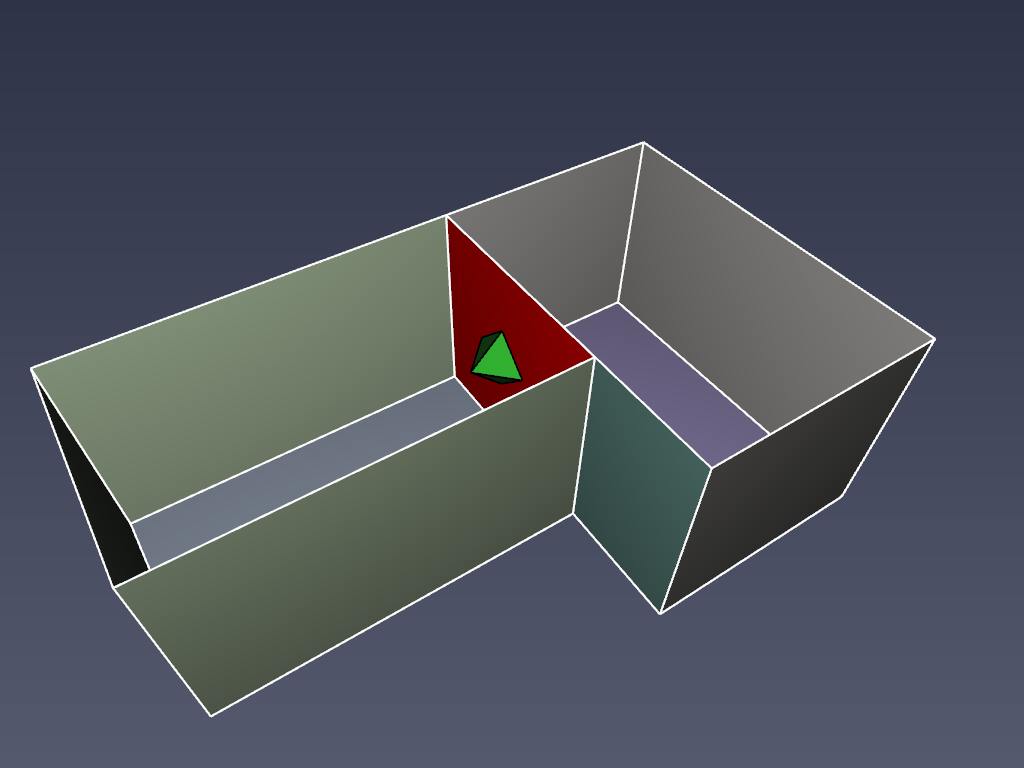
The 3D mode uses snapping in all three dimensions, causing tool properties to be interpreted more loosely. The drawing plane and depth properties for a drawn object are context-sensitive in 3D mode. When using tools such as the Flow Path tool, the first clicked point determines the drawing plane. If, on this first click, another object is snapped to, the drawing plane is set at the Z location of that snap point. The tool properties' drawing plane is only used if nothing is snapped to on the first click.
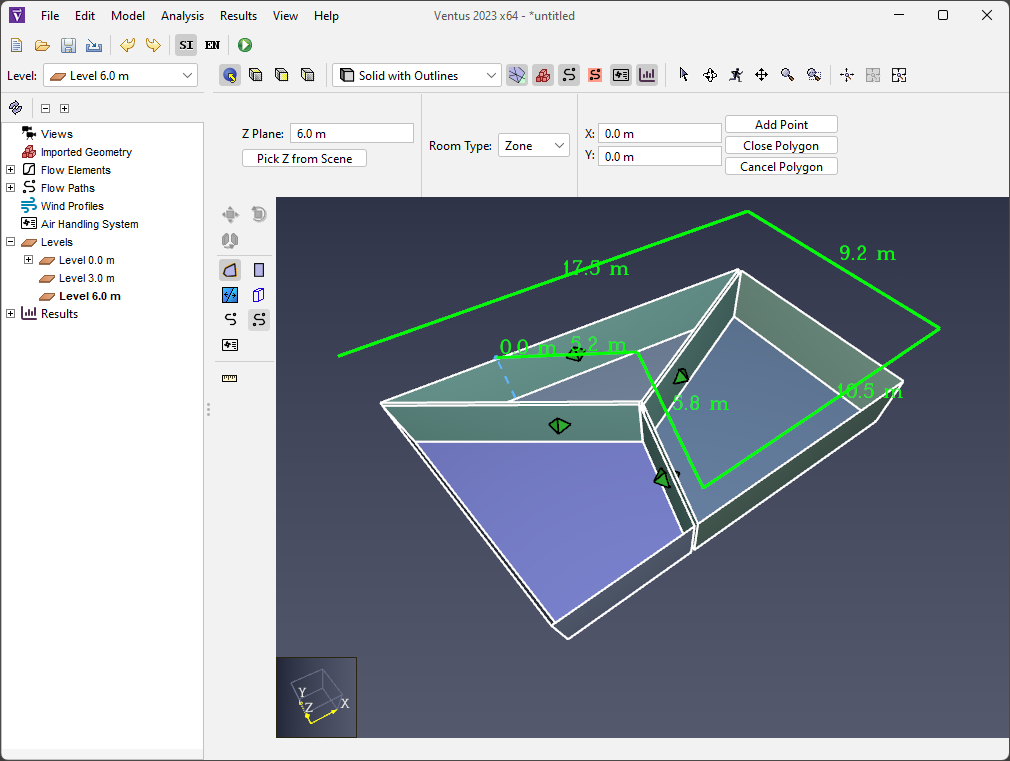
Once the drawing plane for a tool has been established by moving the cursor to a general position, a dotted line will appear and show how the snapped point was projected to another plane, in helping determine an accurate position. For instance, Figure 8 shows a new Flow Path being drawn to a side wall of the zone.
Snapping is one way to precisely draw and edit objects. It is the process of finding some element in the scene, such as a vertex or edge close to the cursor, and snapping the cursor to that element like a magnet.
In Ventus, snapping can be performed against objects in the model and orthographic constraints. These objects include Imported Geometry. The 2D mode additionally provides a sketch grid and polar (angle) constraints. If a snap point is found, an indicator dot, shown in Figure 9, will appear at the snap point.
By default, snapping is enabled. It can be disabled by holding ALT on the keyboard while using a drawing/editing tool.
Ventus provides a user-defined drawing grid, or sketch grid, in 2D mode.
When a new model is created, the sketch grid is visible and can be snapped to in 2D mode.
The default spacing for the divisions is 0.5 m, but can be changed by going to the View menu and clicking Edit Snap Grid.
To disable grid snapping, on the View menu uncheck Show Snap Grid.
All objects displayed in the model can be snapped to when using the drawing/editing tools. There are three basic categories of geometry that can be snapped to on objects: faces, edges, and vertices. Objects can have any combination of types. If there are multiple types close to the cursor, Ventus will give vertices precedence over edges and edges precedence over faces.
Constraints are dynamic snapping lines that are only visible when the cursor is near them. They appear as infinite dotted lines that extend from the most recent relevant clicked point when using a multipoint tool.
Ventus contains two types of constraints:
15 degree increments from the current view’s local X axis.If the cursor is currently snapping to a constraint, that constraint can be locked by holding SHIFT on the keyboard. While holding SHIFT, a second dotted line will extend from the cursor to the locked constraint (the first dotted line). This is useful for lining up objects along a constraint with other objects.
Snapping behavior may change depending on which modeling tool is selected and whether a 2D or the 3D mode is active. If the 3D mode is active, the cursor will snap to a 3D coordinate, which may then be further restricted by the tool. Most tools will indicate the snapped position in the status bar at the bottom of the modeling panel.
Snapping may be a slow operation in complex models. In these cases, asynchronous snapping is used to keep the cursor and application responsive while the snapping operation takes place in the background. During asynchronous snapping, a wait cursor will appear at the cursor crosshairs while the snapping completes. While this takes place, either keep the cursor still to allow the current snapping operation to complete or move the cursor to abort the operation and snap to a different location. Asynchronous snapping can be disabled by unchecking File→Preferences→Enable asynchronous snapping. Note that if it is disabled, the cursor may briefly hang and the application will become unresponsive while these long snapping calculations take place.
Ventus provides the capability to save and recall view state from the Workspace in an object called a View that will be shown in the Object Tree.
There can be multiple views in a model, but at any given time, there is always one active view. A new model will always start with one default view that has no view state associated with it. State can be added to the view as described in the section Viewpoints.
Views are managed in the Object Tree. From there, they can be created, deleted, grouped, rearranged, etc.
A view can be created in one of the following ways:
This will add a new view to the model, saving the current camera viewpoint into the new view. The new view will become the active view.
To delete a view, select it in the Object Tree and in the Edit menu, select Delete. A view can only be deleted if it is not active.
To activate a view, perform one of the following:
Activating a view will restore all its saved state as described in the following sections.
View settings can be copied or moved between views. To copy settings select Copy, located in either the Object Tree or in the Edit menu. To paste the settings to another view, select the desired target view and in the Edit menu select Paste. To move settings from one view to another, in the Object Tree, drag the setting to the desired view.
Each view can have one viewpoint associated with it. A viewpoint includes the 2D or 3D camera’s position, orientation, zoom, and camera type (3D versus 2D). When a viewpoint is saved, the current navigation tool is also saved with the view (Orbit, Roam, etc.). A viewpoint appears in the Object Tree as a child item of a view and is labelled Viewpoint.
A viewpoint is automatically saved to newly created views. A viewpoint can also be explicitly saved in one of the following ways:
The scene camera can be reset to a viewpoint in one of the following ways:
A viewpoint can be removed from a view by selecting the item, Viewpoint, in the Object Tree and deleting it.
When a view with a viewpoint is activated, the following occurs:
To begin drawing or editing with a tool, the user can single-click the tool from the toolbar. Once the tool has finished drawing/editing its object, the last-used navigation tool is automatically selected.
If the user would like to create several objects with the same tool in succession, the desired tool can be pinned by clicking the tool’s button twice.
The button will show a green dot when pinned (![]() ).
).
Every time the same tool button is clicked, the pinned state of that tool will be toggled, so clicking the button again after pinning will disable pinning (![]() ).
).
At any time, the current drawing/editing tool can be cancelled by pressing ESC on the keyboard. This will also cancel pinning and will revert to the last-used navigation tool.
Most drawing/editing tools require at least two points to be specified to complete its action, such as drawing the points for a polygonal room or defining a Flow Path between walls.
These tools can operate in two modes
While using any of the drawing tools, the mouse can still be used to zoom or pan the camera:
When drawing with many tools, Ventus will render dimension labels in the 3D view to aid in drawing geometry to scale. These labels act as guides when drawing, and are particularly useful when working with the Snap Grid described in Snapping.
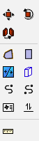
Ventus provides several drawing and editing tools. These tools are located on the drawing toolbar on the left side of the Workspace as shown in Figure 11.
The sections referenced below provide more detail on the specific tools available.
For each tool there are often two ways to create its object.
The Property panel will update the graphical preview immediately to reflect changes in the input. This allows fine-grained control in creating the object.
Drawing can be performed in both the 2D and 3D modes. The 3D mode allows the user to see the model from any angle, but most tools restrict drawing to the X-Y plane. The 2D modes completely restrict drawing to the XY, Y-Z, or X-Z plane, and they also display an optional snap grid. The snap grid size can be set under View › Edit snap grid spacing, and it can be turned off by deselecting View › Show Snap Grid.
Ventus provides a variety of view options for displaying both model geometry and imported geometry that can also aid with drawing. This includes options for rendering geometry, coloring zones, and setting the transparency of zones.
Often it is desirable to turn off the display of selected objects, for example, to hide a roof of a building in order to visualize the interior. In any of the views, right-click on a selection to obtain the following options:
In the toolbar above the Properties panel in the Workspace, there is a drop-down as shown in Figure 12 and buttons as shown in Figure 13 that control how geometry is rendered.
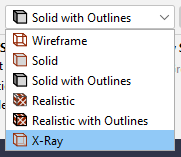

From left to right in Figure 13, the buttons are:
Models can be created using either English or Metric units. To change units, select the preferred unit system via the View › Units menu, or by using the SI/EN Unit System buttons shown in Figure 14. Ventus will automatically convert your previously input values to the Unit System you select.
Levels are the primary method of organization in Ventus. At their most basic level, they are simply groups zones can be placed, but they also control the drawing plane for tools and filtering of imported geometry.
In every Ventus model, at least one level must exist, and at any given time, there is one active level. Whenever any zone object is drawn, it will either be placed in the active level or a subgroup of the active level.
By default, when a new model is started, there is one level at Z=0, and additional levels are either created automatically depending on where the geometry is drawn or manually created.
In addition, new zones are automatically sorted into the appropriate level when drawn.
When nothing is selected in the model and no tools are active, the Level Creation panel is shown, as in Figure 15. This panel controls the automatic creation of levels and automatic sorting of new objects into levels. It also provides some options for level view and selection.
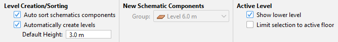
The following scenario demonstrates how objects are organized when auto-sort and auto-level-creation are enabled (organization of the model is shown in Figure 16):
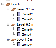
In this example, only Zones were created. The levels were automatically created, and the Zones were automatically sorted into the appropriate ones.
Automatic levels can be created and Zones sorted into the levels by performing the following:
There are two other options in this dialog:
By default, the name of the level is Level \(x\) where \(x\) is the working plane of the level.
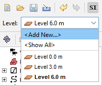
To change the active level, click the level drop-down box as shown in Figure 17, and select the desired level. This will make that level active and all other levels non-active.
Whenever the active level is changed, the following additional changes take place in the model:
To show all levels click the level drop-down box as shown in Figure 17, and click <Show All>.
This will additionally show all sub-objects of the levels groups, and it will set the import filter to the union of all the levels' filters.
To edit a level’s properties, first select the desired level. The Properties Panel as shown in Figure 18 will update, showing the level’s name, its Working Z location, and the Z clipping planes (Z Min Filter and Z Max Filter) for imported 3D geometry.
It also shows some statistics of the level including the total area of the level (Area).
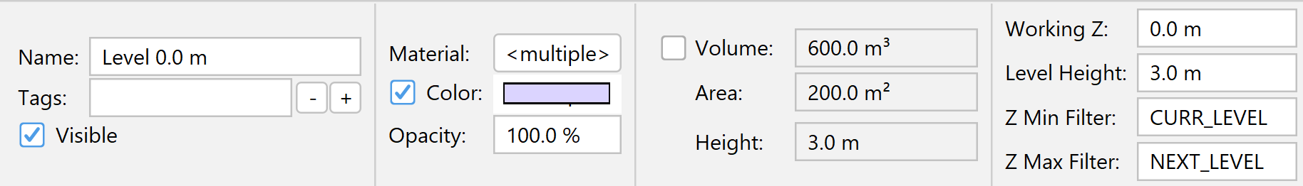
Controls the X-Y plane on which new rooms, walls, and airflow objects are drawn.
CURR_LEVEL.
If it is CURR_LEVEL, then the clipping plane is set to the working Z location if there are any levels below this level or \(-\infty\) if there are no levels below.NEXT_LEVEL.
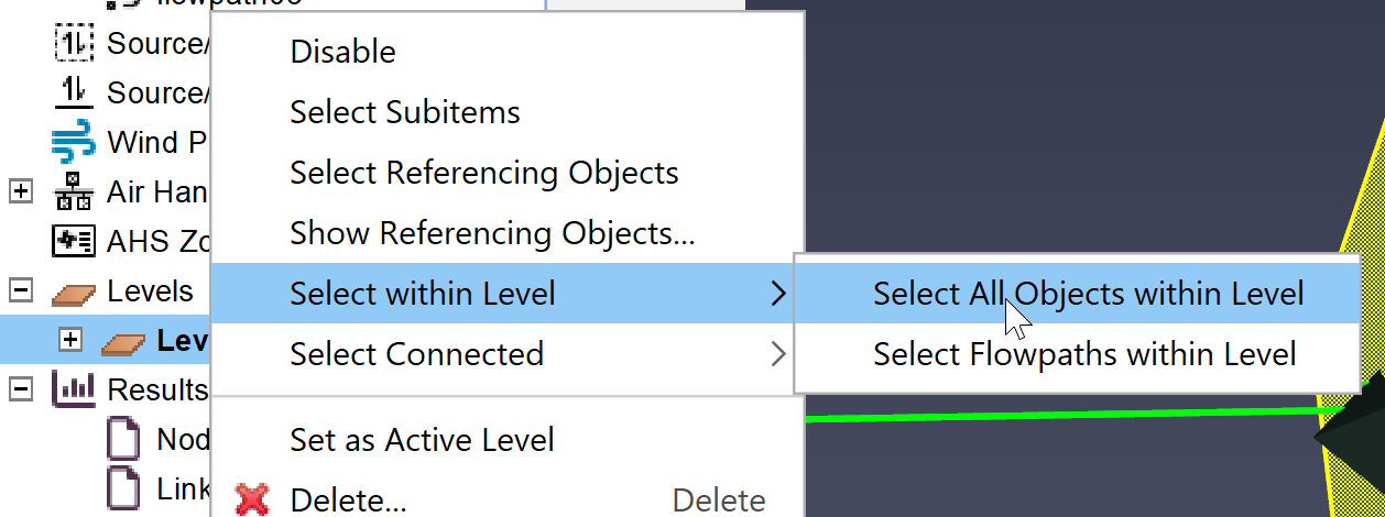
If it is NEXT_LEVEL, then the Z plane is set to the working Z plane of the next higher level if one exists, or \(+\infty\) if there are no higher levels.Because many flow network objects (e.g. AHS Zone Points, Flow Paths, and Sources/Sinks) are not grouped in the Object tree under Levels, efforts have been made to provide users with methods to find and select them quickly.
The Results Panel (Results Panel) provides the ability to quickly observe and filter run results such as to perform an analysis of a specific shaft.
To display the Results Panel select one of the Result tabs from the right-hand side of screen. To hide the Results Panel, click the open results tab again.
The Properties panel lies immediately above the 2D/3D Workspace.
As mentioned in 2D/3D Workspace, the Properties panel is selection context-sensitive. When nothing is selected in the model and no tools are active, the Level Creation panel is shown (as in Figure 15 from Automatically Creating Levels). When an object is selected, the Properties panel will update to display details for that object, as in Figure 20.
Similarly, when a tool is selected, the Properties panel will update to capture input for that tool.
Ventus relies heavily on the idea of selected objects.
For almost all operations, the user first selects an object(s) and then changes the selected object(s).
The Selection/Edit Objects (![]() ) is most commonly used to select objects.
) is most commonly used to select objects.
Once objects have been selected, the user can modify the object using the menus.
A right-click on a selection displays a context menu. This menu includes the most common options for working with the object. The user may also right-click on individual objects for immediate display of the context menu.
While it is simple to select an individual object from either the Object tree or the 2D/3D workspace, doing so for every single object to edit can be cumbersome. Several tools are available to find and select multiple objects at once.
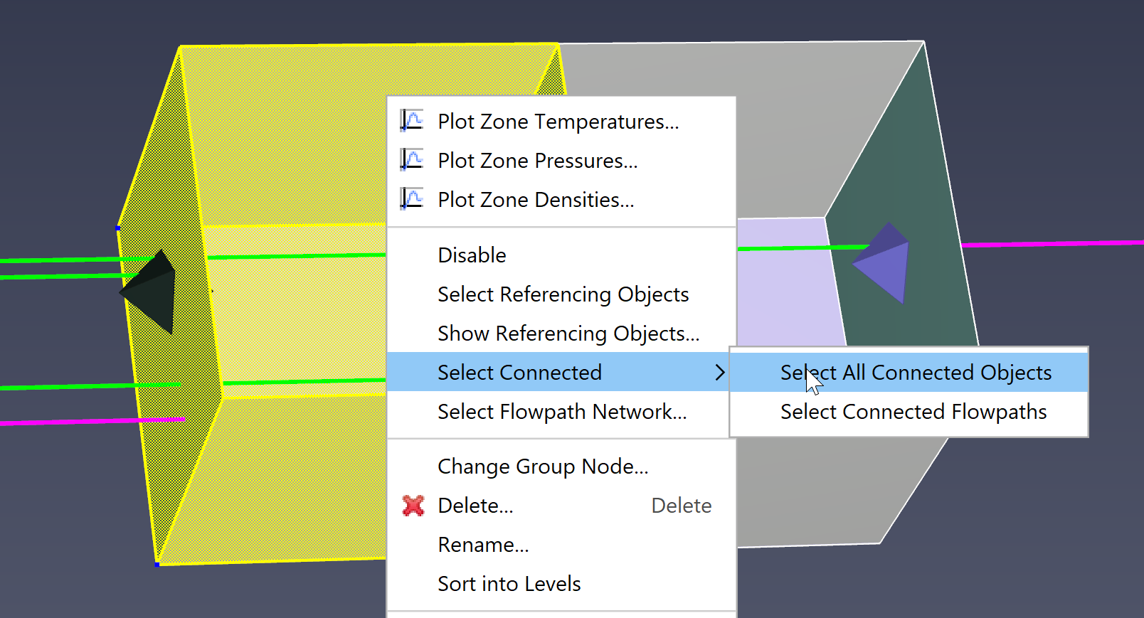
When analyzing the results of a Ventus simulation it is often important to assess a group of Flow Paths connecting to a single volume, such as a Mechanical, Electrical, and Plumbing (MEP) shaft. The search starts at a Zone of interest, and searches through connected Zones based on a specified Flow Element representing connections within the Zone.
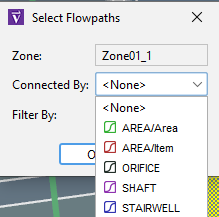
This search can be used in conjunction with Tags to generate a shaft report.
Most models can have complex relationships between objects, with some objects referencing others. In these cases, it can often be helpful to start at the referenced object and see which objects are referencing it.
Right-click the referenced object and choose Select Referencing Objects.
Right-click the referenced object and choose Show Referencing Objects. This opens the floating Show Referencing Objects dialog, which displays each of the referencing objects in a list.
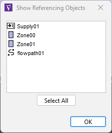
Objects in the list have their selection state synchronized with the selection in the Object panel and the 2D/3D Workspace. This includes the ability to right-click an object in this tool and access the object’s context menu.
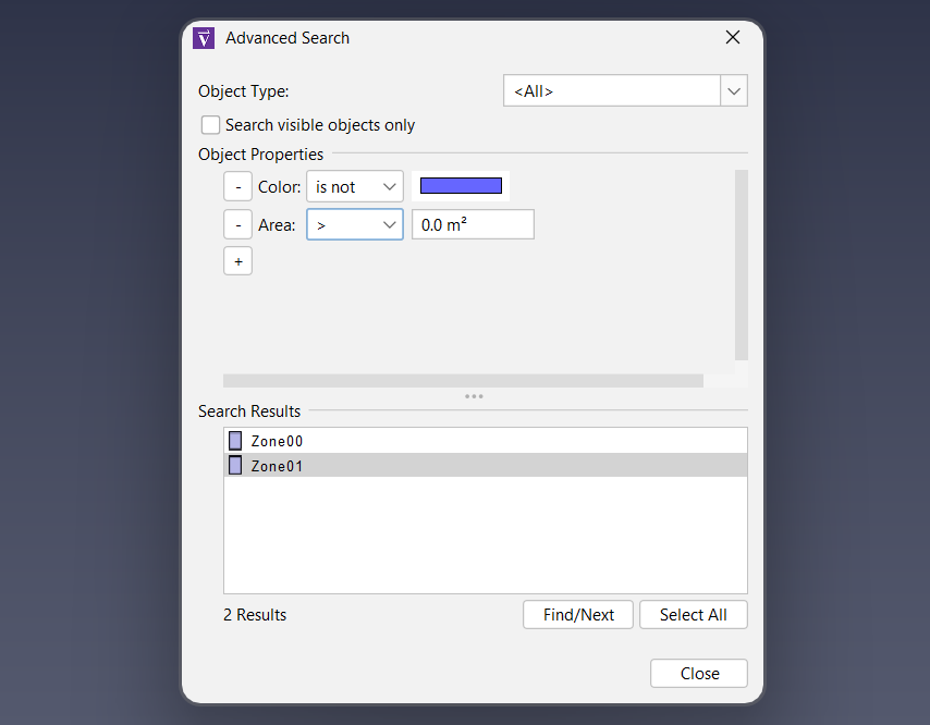
List of properties objects must match. Returned objects must support all properties in this list, and their values must match the listed criteria for all properties.
The plus (+) button can be used to add a new property to this list. This will open the Add Search Property dialog which prompts the user to select a property to search by from a list of properties supported by the currently selected Object Type. This list of properties is text-searchable.
The minus (-) button, next to each property in the list, can be used to remove that search property from the list. If the user selects a different Object Type, search properties which aren’t supported by that object type will be removed.
!= a number.Nearly all geometric objects can also be graphically edited in the Workspace with Select/Edit Objects (![]() ).
).
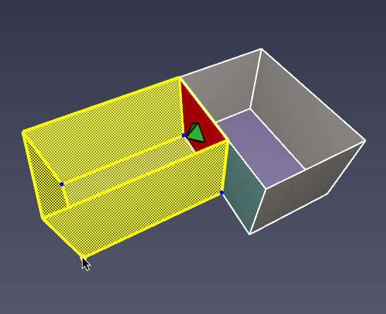
Editing is performed through an object’s editing Handles. Handles appear on an object either as a blue dot as shown in Figure 26 or a face with a different color. The dots indicate a point that can be moved in either two or three dimensions. A discolored face indicates that a face can be moved or extruded along a line.
Double-clicking on an object opens the appropriate dialog for editing the object properties, when such a dialog exists.
As objects are created via the drawing tools, geometry import, manager dialogs, and Copy / Paste, the names assigned by Ventus can become increasingly complex. After some time it may be desirable to change many thousands of object names to make the model more clear.
To open the Rename dialog, right click one of the selected objects in either the workspace or in the Object Panel and select Rename….
For more complex renaming scenarios, you may check the Rename with Template checkbox.
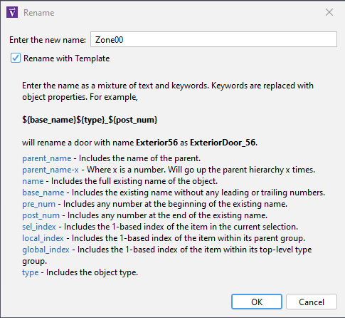
When the Rename with Template checkbox is selected, you may create a name as a mixture of both text and keywords. Keywords are uniquely interpreted for each of the selected objects based on the object’s properties. Using this approach a large set of mixed-type objects can all be renamed according to a standard syntax.
For example: ${base_name}${type}_${post_num}
will rename a door called Exterior56 to ExteriorDoor_56.
The full set of available keywords are as in Table 3.
name | The existing name of object |
base_name | The existing name of the object without any leading or trailing numbers |
parent_name | The name of the parent object |
parent_name-x | Where x is a number. Will go up the hierarchy x times |
pre_num | Any number at the beginning of the existing name |
post_num | Any number at the end of the existing name |
global_index | The 1-based index of the object within its top-level type group |
local_index | The 1-based index of the item within its parent group |
type | The object type |
Each of these keywords are detailed in the Rename dialog dropdown.
To make it easier to work with name templates, the keyword names in the dialog work as hyperlinked buttons as in Figure 27. Clicking one of the keyword buttons will inject the keyword directly into the editor dialog at the current caret location.
Ventus provides a variety of tools to transform geometry objects. With the transform tools, users can move, rotate, and mirror objects.
This tool allows the user to move selected objects to a new location, or to create and move a copy of the selected objects.
This tool allows the user to rotate selected objects, or to create and rotate a copy of the selected objects.
The selected objects will be rotated about the Rotation Axis at the Rotate Base by the Angle specified.
The default Rotation Axis about which objects are rotated for each view are
The mirror tool allows selected objects to be mirrored across a plane, or to create a mirrored copy of the selected objects.
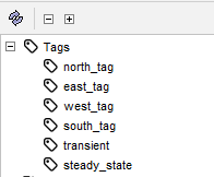
Any number of custom Tags may be added to identify and organize objects with common characteristics. Most objects in the Object panel support tags. Once added, the given Tag will also appear in its own group in the Object panel. Most non-group objects in the Object panel support tags. Once added, the given Tag will also appear in its own group in the Object panel.
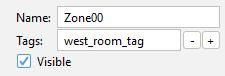
Tags are assigned in the Property panel. A Tag will be created for each unique character string separated by spaces or other delimiter characters.
If multiple objects are selected, the Tag editor will display as <mixed>. Editing the Tag field in this state can potentially cause unexpected changes.
To work around this, the Tag editor includes custom buttons for adding or removing Tags in a mixed selection state.
The + button will launch an editor where you may enter the Tags you would like applied to each selected object.
The - button will launch an editor where you may enter the Tags you would like to remove from each selected object.
One of the main purposes of Tags is to quickly find and identify related objects. Ventus provides several ways to quickly find tagged objects.
To find tagged objects using the Find dialog, perform the following:
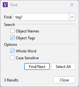
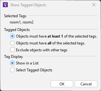
tag1 and tag2, the chosen objects will have either tag1 or tag2 or both tag1 and tag2.tag1 and tag2, the chosen objects will have both of the tags.tag1 and tag2, and an object contains these tags but also contains tag3, it will be excluded from the result.
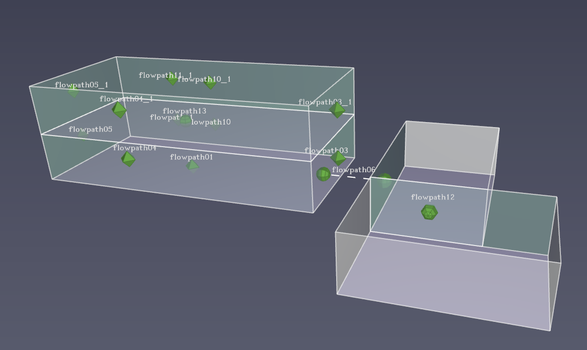
This may be useful, for instance, to find objects that contain exactly the selected tags and no more.Object labels help the user to quickly see what the name of the Flow Path is without having to select each one.
The Size, Opacity, and Color of the labels can be configured in General Preferences.
The labels can be hidden or shown with the view tool ![]() (See Render Options).
(See Render Options).
Libraries of Flow Elements, Wind Profiles, and Air Handling Systems can reduce errors and speed the creation of new models. The user can import data from the library into a new model.
You can create and manage your own libraries for data that you commonly use. A library is a single file that can contain a single category of objects.
<Object> Libraries dialog, use the Load Library… button to choose the <object> VLIB file.
This loads the objects.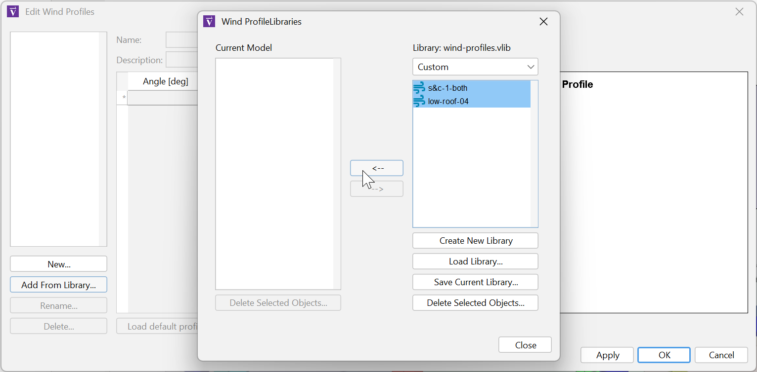
Ventus preferences can be set by going to the File menu and choosing Preferences. Any changes to the preferences will be set for the current Ventus session and be remembered the next time Ventus is started.
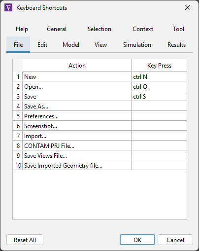
The dialog is split into sections similar to those used in the Ventus toolbar menus. There are additional tabs for shortcuts related to tool activation, object selection, and context-sensitive actions.
To change the key binding for an action, click the value in the Key Press column. This launches an editor window (Figure 35) with four options.
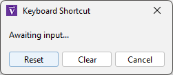
Some keyboard shortcuts are used by Java UI components. If a shortcut does not result in the expected behavior, it may be in direct conflict with a preexisting Java shortcut. It is best practice to avoid these conflicts (Default Swing key bindings).
testing.vnts for example) becomes corrupted, then you can find the file that includes a tilde like testing.vnt~.
This file is sometimes preferred if you have a crash, as it will be the most up-to-date version of your work before your crash.
If it cannot be opened or results in an immediate crash, there is another backup file described next that is the second-best option.
The default setting enables this feature and saves every 10 minutes.
In some cases, when working with large models, this can cause unexpected delays during the save and some users prefer to disable the feature and save manually.testing.vnt~.
Rename (recommended) or delete your current working file, then change the file extension on this backup file, changing the tilde in the extension (.vnt~) to a s character to get .vnts.
You can now open the new backup-testing.vnts file as you normally would.These preferences define advanced 2D and 3D display properties. They can be used to improve display performance on complex models, but they tend to create problems for some older graphics cards, including crashing. For this reason, they are turned off when running in safe mode.
Ventus stores data related to user preferences in a file called Ventus.props. By default, this file can be found in one of the following locations.
%APPDATA%\Ventus\Ventus.props%PROGRAMDATA%\Ventus\Ventus.props
If at least one of these files exists, Ventus will use it to load the user preferences.
If both files exist, Ventus will load user preferences from both files, giving preference to the file located in the APPDATA folder.
This way the preference file located in the PROGRAMDATA folder can be shared among multiple machines, and the file located in the APPDATA folder on each machine overrides the shared settings.
The PROPS file is stored in a plaintext format, and can be viewed or edited with any conventional text editor.
While it is not recommended to edit the file directly, some troubleshooting techniques may involve deleting the PROPS file so that a new one can be created from scratch by Ventus.
Configurations for hotkeys in Ventus is stored in a separate file named key bindings.json located in the APPDATA folder.
To select a Default, Black Background, White Background, or Custom color scheme, on the View menu, click Color Scheme.
The custom color scheme is defined in the Ventus.props file in the Ventus installation directory (For Windows 10+ look in %USERPROFILE%\AppData\Roaming\Ventus\Ventus.props while some older operating systems use C:\Program Files\Ventus).
Ventus.props fileColors.Custom.axis=0xffff00 Colors.Custom.axis.box=0x404040 Colors.Custom.axis.text=0xffffff Colors.Custom.background=0x54596E Colors.Custom.background2=0x2E3348 Colors.Custom.boundary.line=0xffffff Colors.Custom.origin2D=0x737373 Colors.Custom.snap.point=0xff00 Colors.Custom.snapto.grid=0x404040 Colors.Custom.snapto.points=0xc0c0c0 Colors.Custom.text=0xffffff Colors.Custom.tool=0xff00 Colors.Custom.tool.guides=0x7c00
Ventus.props fileAll selections and model edits can be undone and redone using the Undo (![]() ) and Redo (
) and Redo (![]() ) buttons, as well as the shortcuts CTRL+Z and CTRL+Y, respectively.
The shortcuts CTRL+SHIFT+Z and CTRL+SHIFT+Y will skip selection history and revert or continue to the next model edit.
) buttons, as well as the shortcuts CTRL+Z and CTRL+Y, respectively.
The shortcuts CTRL+SHIFT+Z and CTRL+SHIFT+Y will skip selection history and revert or continue to the next model edit.
Alternately, the drop-down tab adjacent to the Undo (![]() ) and Redo (
) and Redo (![]() ) buttons or the Edit→Undo and Edit→Redo menu can be used to view your Undo or Redo history and jump to a specific point.
) buttons or the Edit→Undo and Edit→Redo menu can be used to view your Undo or Redo history and jump to a specific point.
The size of your history can be changed in File→Preferences→Undo/Redo History. History for model edits is limited by that preference, while history for selection-only changes has double that limit.
Select an object to copy, then either use CTRL+C or Edit→Copy to copy. Alternately, right-click on an object to display the context menu with Copy.
Either use CTRL+V or Edit→Paste to paste a copy of the object. Alternately, right-click on a destination to display the context menu with Paste.
By running two instances of Ventus, you can copy objects from one model and paste them into a second model. If the copied objects are dependent on other objects, such as a Flow Path that is dependent on a flow element, and those dependencies do not already exist in the second model, these properties will be included as part of the paste payload.
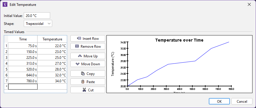
Some objects in Ventus have properties which can be given a Schedule over time. A Schedule editor dialog (Figure 36) can be used to edit these Schedules.
In some parts of the Ventus user interface, individual single-value parameters can be entered as a list. In these cases, entering multiple values causes Ventus to run multiple scenarios as a batch.
When running a multiple scenario model, Ventus will automatically calculate the Cartesian product of scenario parameter assignments, name the scenarios based on the parameter values, run individual simulations for scenario, and show all results in the Object Tree.
Examples where parameters can be entered as multiple scenario parameters are the Ambient Temperature and Wind Direction values in the Weather and Wind dialog, on the Weather tab.
Images of the current display can be saved to a file by opening the File menu and clicking Snapshot. The user can specify the file name, image type (PNG, JPG, TIF, BMP), and the resolution. A good choice for image type is Portable Network Graphics (PNG).
Several files are used when performing airflow analysis using Ventus. These include the Ventus model file, the CONTAM input file, and CONTAM output files. This section describes how to load and save files in the formats supported by Ventus.
When Ventus is started, it opens with an empty model. You can close the current model and create a new empty model by opening the File menu and clicking New. Ventus always has one (and only one) active model.
The Ventus model file (referred to as VNTS, with the extension .vnts), is stored in a binary format that represents a Ventus model. The Ventus model contains all the information needed to write a CONTAM input file. This format is ideal for sharing your models with other Ventus users.
A list of recently opened files is also available. To open recent files, on the File menu, click Recent Files, then click the desired file.
Ventus has an auto-save feature which stores a copy of your current model every 10 minutes. This file is automatically deleted if Ventus exits normally, but if Ventus crashes, you can recover your work by opening the autosave file. It can be found either in the same directory as your most recent VNTS file, or in the Ventus installation directory if your model was unsaved.
Ventus provides tools to help the user rapidly create and organize model geometry. Geometry can be created by using the drafting tools in the Workspace as discussed in Tools.
The user can also organize the model by creating Levels and Groups. In addition, the user can assign background images to Levels to aid in drawing Zones and Ceilings.
CONTAM calculations are performed between zones. A Zone is a volume of air that is typically contained within the bounds of a room. Zones are the basic units between which airflow is calculated. Zones have properties that determine airflow, including air temperature and pressure, which are used to calculate density.
In addition to Name, Material, Color and Opacity, the following properties are available on the Properties Panel (Figure 38) for Zones

Zones in Ventus are created using the Room Tools. The volume of a Zone is determined by the floor area of the room and its ceiling height.
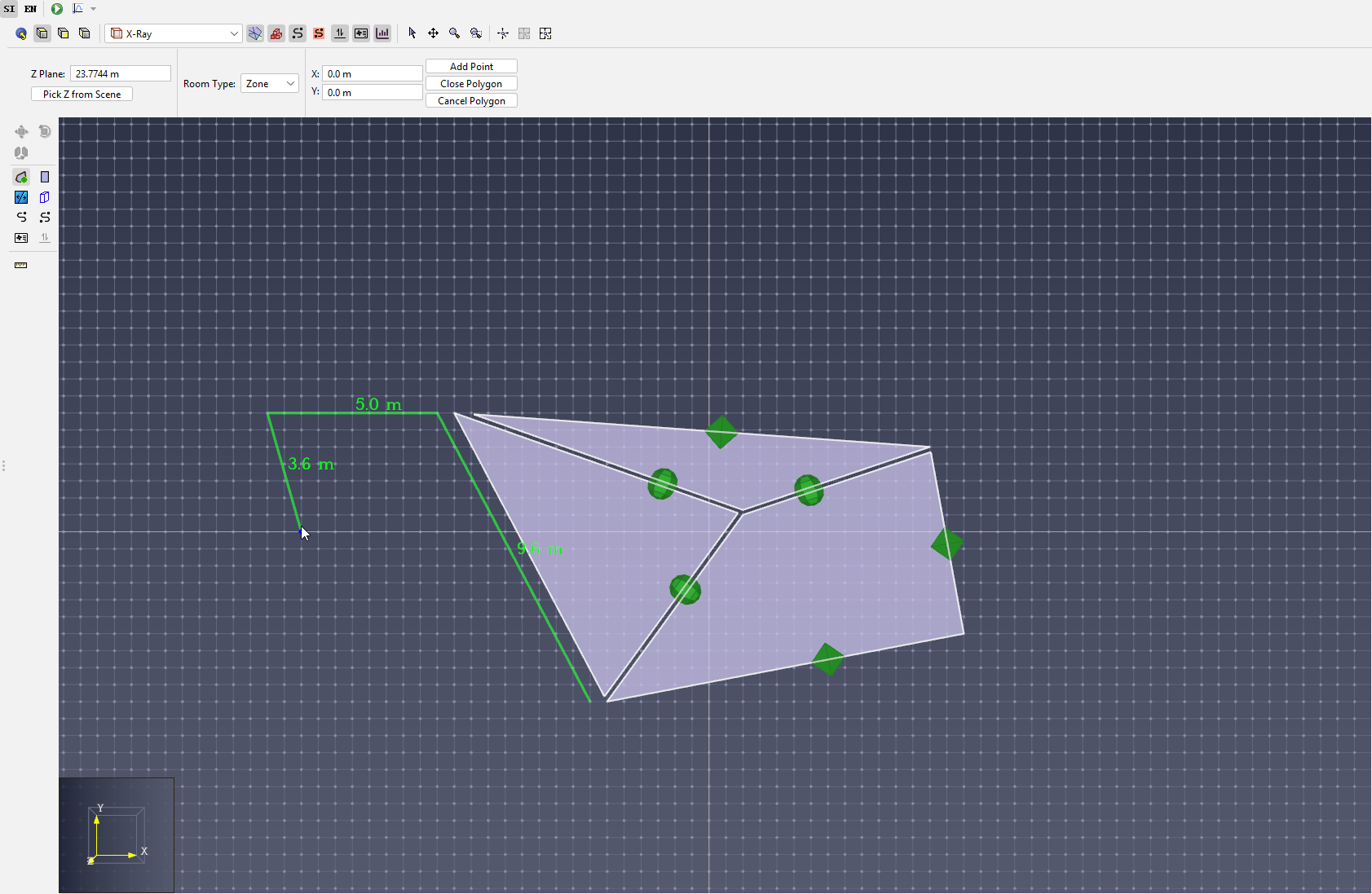
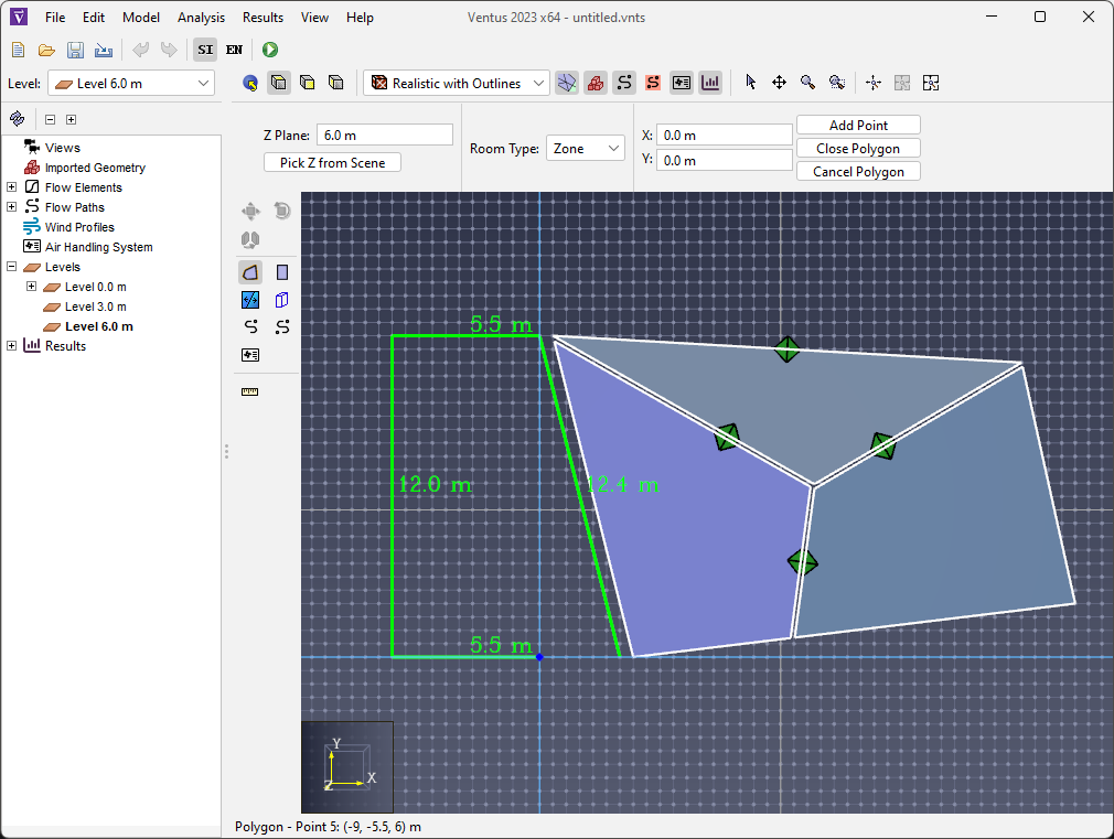
The Polygonal Room tool ![]() allows for the creation of complex shapes with any number of vertices (Figure 39).
allows for the creation of complex shapes with any number of vertices (Figure 39).
Left-click anywhere in the model to set the first point, and continue left-clicking to add more points to the polygon. When at least three points are defined, right-clicking will close the polygon and complete the shape.
Alternatively, X,Y coordinates can be entered from the keyboard with the Add Point and Close Polygon buttons from the Property panel.
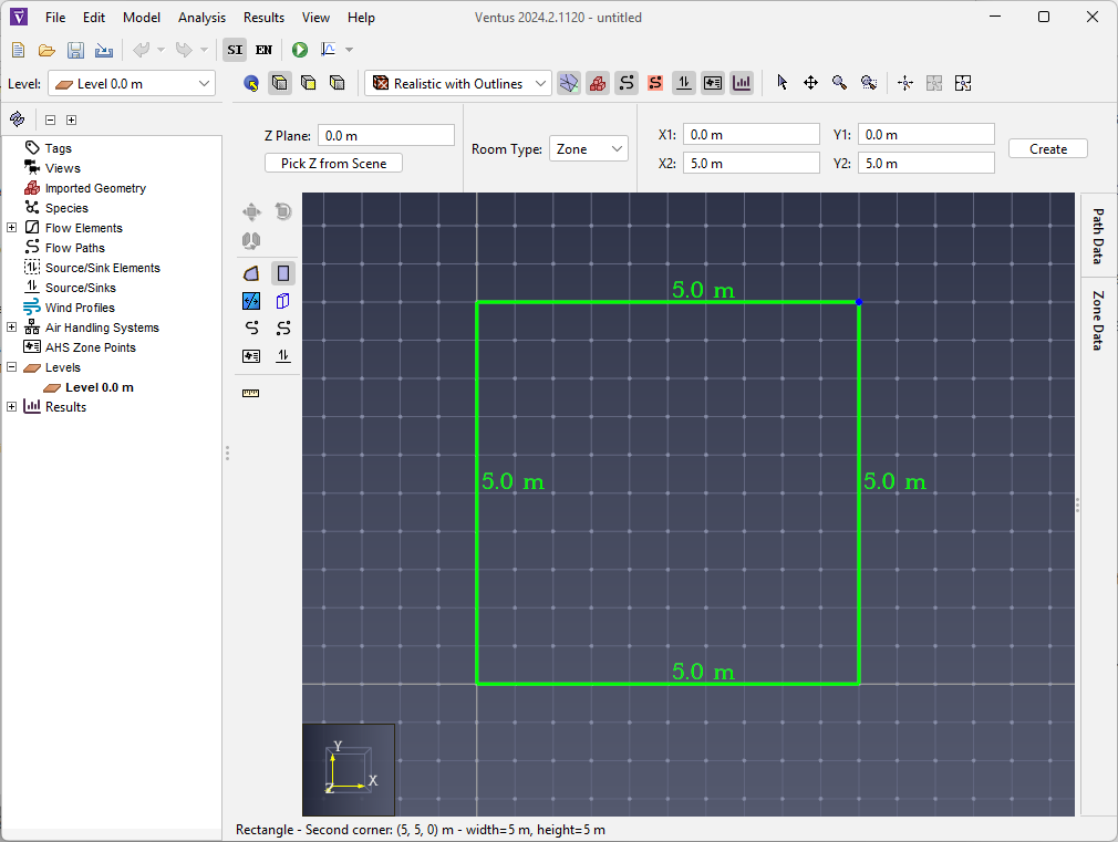
The Rectangular Room tool ![]() creates simple rectangular geometry by left-clicking two points in the model (Figure 40).
creates simple rectangular geometry by left-clicking two points in the model (Figure 40).
The rectangular area can also be created by entering coordinates for two points in the Property panel and clicking Create.
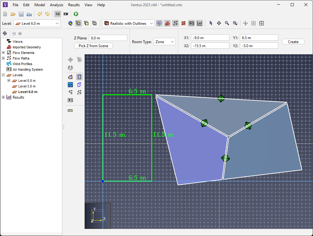
In addition to creating new areas, both of these tools can be used on existing geometry to create negative areas. Creating new geometry over existing areas removes any interfering portion from those areas. The newly created geometry can then be deleted, leaving the negative space behind.
Ventus supports the concept of an ambient zone.
The Ambient Zone is not bounded, but instead defines the properties of the outdoor air that surrounds bounded zones. The pressure and temperature of this Ambient Zone can be set in the Weather and Wind dialog.

Ceilings are drawn with the same tools as Zones. (Zone Tools)
Wall tools are available in Ventus to split existing rooms into more than one zone.
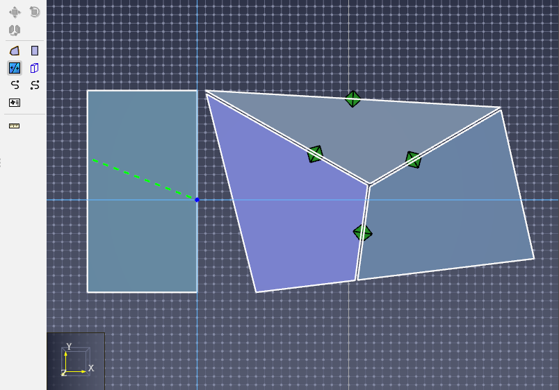
Thin, internal walls or boundaries can be added to zones with the Thin Wall tool ![]() .
.
To use this tool, click two points in the model as shown in Figure 42. Ventus will attempt to connect these two points with an internal boundary edge.
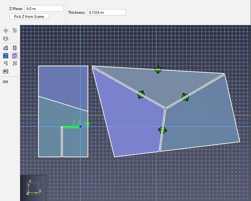
The Thick wall tool ![]() can also be used to add internal walls or boundaries to zones (Figure 43).
It differs from the thin wall tool in that it operates by subtracting area from any room that lies in its specified X-Y plane.
This subtraction will generally leave a gap in space in the Zone the wall tool is separating.
This gap will be determined by the Thickness property of the wall tool, which can be set by the user.
can also be used to add internal walls or boundaries to zones (Figure 43).
It differs from the thin wall tool in that it operates by subtracting area from any room that lies in its specified X-Y plane.
This subtraction will generally leave a gap in space in the Zone the wall tool is separating.
This gap will be determined by the Thickness property of the wall tool, which can be set by the user.
While Ventus’s tools do not explicitly produce curved walls, they can approximate them by drawing the wall using several straight wall segments.
Ventus provides a Measure Tool (![]() ) to measure distances in the model.
) to measure distances in the model.
To measure a distance, perform the following:
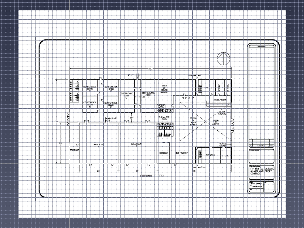
Geometry can be created from Images in Ventus by drawing on top of an imported 2D image, such as a dimensional floor plan.
Background images can be imported by clicking New Background Image on the Model menu.
(0,0,0) in the model.(1,0,0).
As shown in the figure, the A→B vector should be 90 degrees from the X axis.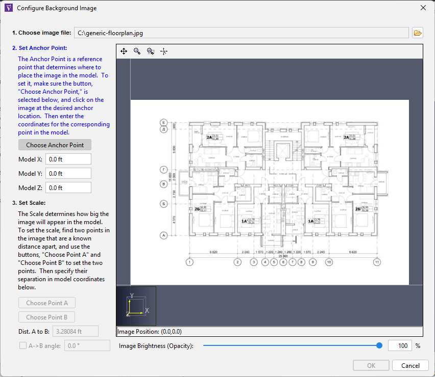
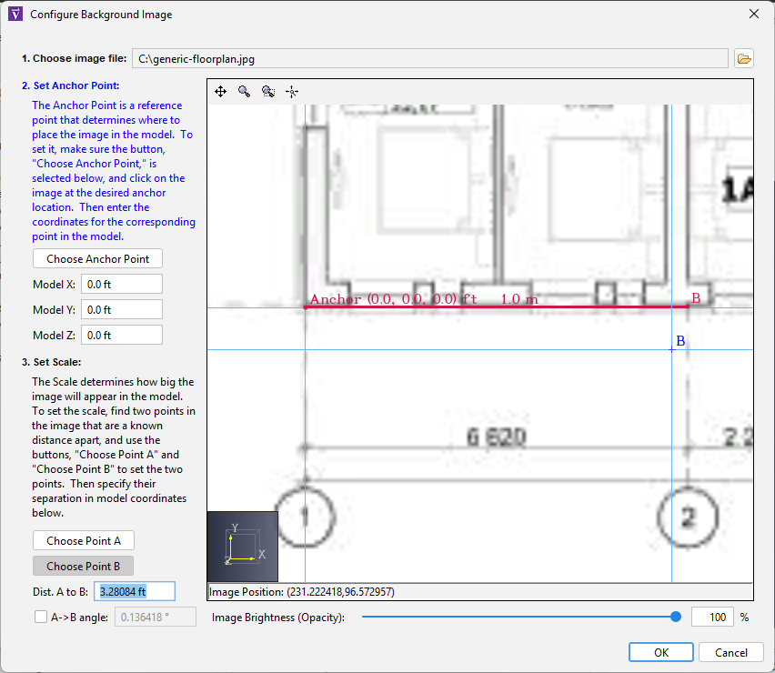
The imported image is added to the Imported Geometry → Background Image group in the Object panel. The image can be edited and deleted from there.
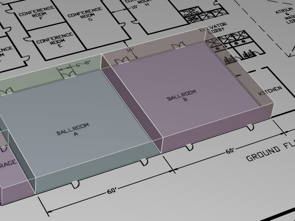
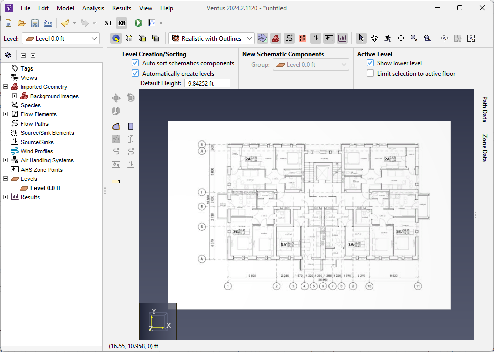
Working with background images requires the user to draw Zones and Ceilings over the background image (Figure 47). Because the drawn Zone geometry will cover the background image(s), it may be preferable to make the Zone transparent. This can be accomplished by selecting the drawn Zones and lowering the opacity in the Property panel. Figure 48 shows a background image with rooms and doors drawn on top, with a lowered opacity for the Zones.
| |
Show/hide can be toggled on and off with the ![]() Show Background Images tool in Render Options.
Show Background Images tool in Render Options.
PDF Files are imported the same as images. See Creating Geometry from Images.
Ventus can import geometry from several CAD formats, including buildingSMART’s IFC format for Building Information Models (BIM), AutoCAD’s DXF (Drawing Exchange Format), DWG, FBX, DAE, OBJ, GLTF/GLB 2.0, and STL files. Each type of file provides a variety of geometry that can either be directly represented as obstructions or as drawing guides in the Ventus model.
This facilitates the ability to import data from several CAD files into one Ventus model. This is useful when there is one blueprint per floor of a building or a 3D building has been split into several sections, each in a separate file.
To import one of these files, under the File menu, select Import and select the desired file.
Unknown.
This selection controls the default settings in the subsequent prompts.
In some cases, Ventus is able to detect whether the file was exported using a SimLab plugin and will select this option automatically.+Y is down.Specular (Basic) workflow, as this is the only workflow supported by IFC and FBX files.
In some cases, however, such as when an FBX file is exported from Unreal Engine, the PBR parameters are packed into the basic specular texture property.
In this case, the following two options can be used to reinterpret the basic specular workflow as a PBR workflow for correct lighting.Metallic (PBR) workflow, even if they are specified in the import file using the Specular (Basic) workflow.
When using this option, the PBR parameters can either be set to constant values or can be reinterpreted from other non-PBR color properties.
For instance, when an FBX file is exported from other software, for each material it might create a single image containing the Metallic, Roughness, and Ambient Occlusion parameters, stored in the red, green, and blue color components, respectively.
It then might set the specular texture in the FBX file to this combined image.
When an exporter does this, there should be accompanying documentation with the FBX file that indicates how these PBR parameters are stored in the FBX file.
When importing the FBX file in the above example, in the import dialog, the Metallic, Roughness, and Ambient Occlusion properties should all be set to From Specular, and the color components should be set to R, G, and B, respectively.Once the file is imported, Ventus creates a hierarchy of groups and objects, such that there is one top group, named after the file. The next levels depend on the imported file type. For non-DWG/DXF files, the structure will mimic the node structure (data hierarchy) in the source file. For DWG/FXF files, the next level contains a group for every layer containing geometry. Under each layer group there are one or more objects representing the entities in the file. The following illustrates the hierarchy as it would appear in the Object Tree:
If the DWG/DXF file contains a block insert and the block contains entities from multiple layers, the block insert is split into several Ventus objects, one for each layer of the block’s originating entities. If all the entities in the block are from the same layer, however, there will be one resulting Ventus object that will belong to the group corresponding to the block’s entities' layer rather than the block insert’s layer.
While Ventus cannot directly import Autodesk Revit files (RVT), there are several ways to export the data from Revit into a file format that Ventus can read. Each method has advantages and disadvantages as discussed below.
C:\ProgramData\Autodesk\Revit\Addins\SimLab\FBXExporter\data\Imported_Textures\#Materials define advanced display properties that can be applied to faces contained in the imported geometry. They are only shown when the Realistic or Realistic with Outlines option is selected, see View Toolbar. Materials can be shared among faces; when a material is edited, all faces referencing that material are updated.
Materials are extracted from a particular set of import file type:
To see materials that have been imported, on the Model menu, select Manage Material Database. The Material Dialog will appear as shown in Figure 49.
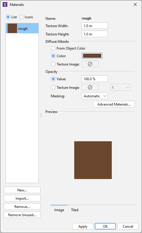
Ventus provides some default database materials.
Most of these materials start with the prefix, psm_ as in PyroSim, a separate Thunderhead Engineering product.
Other materials were either created manually by the user or were imported with a CAD file.
Materials can be added manually by clicking New under the material list. Materials can also be created from an initial texture image on disk by clicking Import. The image is copied into the database directory. Newly created materials are added to the database, and can be used across instances of Ventus.
Materials can be deleted by clicking Remove under the material list. If the material exists in the database, all its associated files in the database directory will also be permanently removed.
The following material properties can be edited from this dialog:
0.5 are drawn as opaque and those with opacity < .5 are not drawn.
The following masking options are available:Additional material properties can be edited by pressing the Advanced Materials button. This will show the Advanced Materials Dialog for the currently selected material.
Most properties in this dialog can be specified as either a constant color/value or as a texture image.
For those properties that represent a single value as opposed to a color, such as the Roughness value for PBR workflow, a dropdown next to the texture chooser can be used to pick which color component is the source of the values.
This is useful when multiple properties are packed into a single image, but in different color components.
For instance, say the PBR parameters, metallic, roughness, and ambient occlusion, are packed into the red, green, and blue color components of a single image.
In this case, the same image can be chosen for the metallic, roughness, and ambient occlusion textures.
The dropdowns next to each texture would be set to R, G, and B, respectively.
The following material properties can be edited from this dialog:
Depending on which workflow is selected, the following additional properties are provided:
ao_inverted = 1.0 - ao_texture).
This is useful when the ambient occlusion texture specifies the amount of occlusion (increasing values lead to more occlusion) rather than amount of visible light (lower values lead to more occlusion).Air can flow between different rooms in a building through a variety of interfaces, including doors, windows, HVAC systems, or the natural leakage between imperfectly sealed walls.
Flow Paths define how air flows between two adjacent Zones in Ventus. They can exist between two regular bounded zones, or between a bounded Zone and the ambient (outdoor air) Zone. They can be defined on the wall or floor of a bounded Zone, or the plane of a Ceiling. Multiple Flow Paths can be defined on a single face.
Flow Elements define the model used to calculate airflow and pressure changes across Flow Paths (Flow Paths). Each Flow Path must specify a flow element; each individual flow element can be used by multiple Flow Paths.
Ventus provides some predefined Flow Elements suitable for common building features, and users are encouraged to create custom Flow Elements. Custom Flow Elements can be saved to a Ventus library file (.vlib).
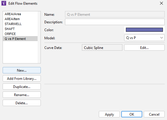
To create, modify, and delete Flow Elements, you can use the Edit Flow Elements dialog. To open the Edit Flow Elements dialog, on the Model menu, click Edit Flow Elements. The dialog in Figure 50 shows the dialog being used to edit a Flow Path element.
Color can also be assigned in the dialog.
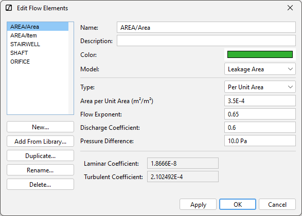
ContamX supports a number of Powerlaw models for modeling mass flow for different types of common building features. Each Flow Element will model one-way flow using one of these Powerlaw models. The general mass flow Powerlaw model is of the form:
\(F = C(\Delta P)^n\)
Where \(F\) is the Mass Flow Rate, \(C\) is the Flow Coefficient, \(\Delta P\) is the Pressure Difference across the Flow Path, and \(n\) is the Flow Exponent. These values are either taken as input or statically derived during the creation of Flow Path elements.
This model is intended for use in modeling orifices that exist on the faces of zones.
The parameters for creating a flow element using the Orifice Area model are:
This model is intended for use in modeling quantified leakage that occurs between rooms due to features in residential buildings.
This model is intended for use in modeling airflow within a stairwell.
This model is intended for use in modeling airflow within a building shaft, typically an elevator shaft or MEP shaft.
These models allow the user to define the relationship between flow rate and pressure drop by providing a set of input points to fit with a cubic spline curve. The fit curve will then define the performance of the flow element.
The Q vs P is the only Cubic Spline model supported in Ventus
\(Q = f(dP)\)
Volume Flow Rate as a function of Pressure Difference. This model is essential when component data is provided in the form of a Q vs P chart (Volume Flow vs Pressure).
Curve input data can be edited from the Edit Flow Elements dialog.
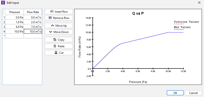
If the input points result in any negative or zero slope values, Ventus will prompt the user to change them.
These models define flow rate based on the pressure difference across the path and the direction of the pressure drop. They would typically be used to model smoke control dampers.
The Self-regulating Vent is the only Damper model supported in Ventus
This model is intended for use in modeling airflow across a path that is regulated by a vent. The model is sensitive to the direction of each Flow Path object.
Paths that utilize fan or forced flow elements are not variable flow links; their flows are specified and not allowed to vary according to the numerical solution techniques.
"This [model] will provide the specified constant mass flow rate regardless of the density of the air being delivered by the fan." (Dols and Polidoro 2020)
"This model describes an airflow element having a constant volume flow rate… if actual conditions during simulation do not match [standard air] conditions, the results will differ from specified flow due to differences in air density." (Dols and Polidoro 2020)
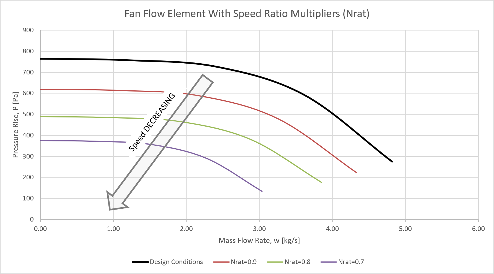
This model allows the user to define the relationship between flow rate and pressure rise (\(- dP\)) by providing a set of input points to fit with polynomial curve in Ventus. The fit curve will define the relationship unless the fan Multiplier Schedule falls below the specified cut-off ratio; below cut-off, the Flow Path switches to an Orifice Powerlaw model with the Equivalent Orifice Area.
Variable Air Volume (VAV) electric fans are often used in building smoke control and airflow management projects. To run the fan at different speeds, always enter normalized fan speeds into a Multiplier Schedule.
VAV Fans in Ventus follow Fan Laws, and the Performance curve can be scaled with the speed ratio, which is equal to the Schedule value (Nrat). The CONTAM User Guide’s Theoretical Background and W.C. Osborne’s Chapter on Fan Operation in Fans are excellent references for understanding fan performance and the Performance Curve Flow Element in Ventus (Dols and Polidoro 2020).
As specified in the CONTAM User Guide:
A two-way flow is driven by the temperature (actually air density) difference between the two zones. When this temperature difference approaches zero the algorithm used for solving the flow tends towards a division by zero problem. To avoid this undefined situation the two-way model reverts to a one-way power law model at this "minimum temperature difference" using the opening size to define the orifice.
(Dols and Polidoro 2020)
In both cases, the local flow calculations consider hydrostatic force across the height of the opening, and the model switches to a one-way Orifice Area flow model at a Minimum Temperature Difference of 0.01 °C.
Remember the lumped parameter model limitations when categorizing airflow, especially in near-fire environments. Neither two-way flow model can account for the increased heat nor concentration of contaminants within a fire upper layer, since there is a single pressure Zone. Only the density is used to modify flows across a vertical opening, and mass transport equations only describe fully mixed Zones.
\(d\dot{m}/d\dot{P} = \dfrac{\dot{m} (\Delta P) - \dot{m}(f * \Delta P) }{f * (\Delta P)}\)
\(H\), the height of the vertical opening
Performs numerical integration to calculate the airflow across the vertical pressure profile.
\(F = W \int{\rho_m V dz}\)
Approximates the total flow with two openings offset from the neutral plane of the opening. This is the same method as the Two Opening Model with 2-way Flow airflow element model in ContamW, where two effective openings are modeled at a vertical distance of \(\dfrac{2}{9} H\) from the center of the opening, using a standard Orifice Powerlaw flow model for each.
The equation for each of the two openings is
\(F = C_d A_o (\Delta{P} \rho)^{n}\)
This model becomes less precise as the neutral plane shifts away from the center of the vertical opening.
Flow paths can be created in Ventus using the Flow Path Tools.
There are two Flow Path tools in Ventus: one point and two-point (![]() ).
A one point Flow Path tool is used to create a Flow Path by choosing one point on a face, while a two-point Flow Path tool is used to create a Flow Path between two Zones through a specified object (usually a wall).
).
A one point Flow Path tool is used to create a Flow Path by choosing one point on a face, while a two-point Flow Path tool is used to create a Flow Path between two Zones through a specified object (usually a wall).

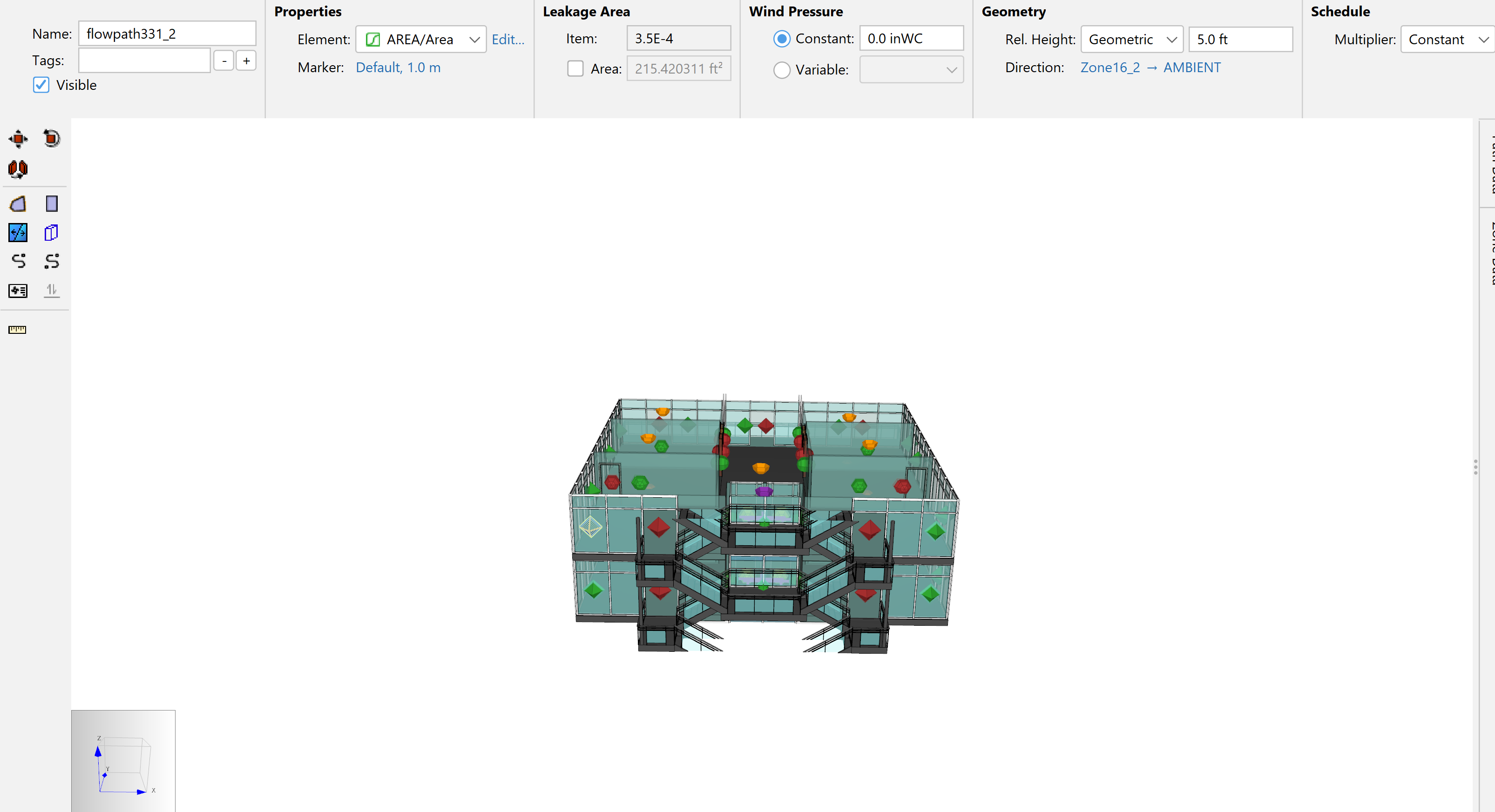
The following properties are available on the Flow Path Panel for a Flow Path
For Powerlaw Models of Flow Elements, describes whether leakage area is defined per-item, per-length, or per-area. Offers a specific multiplier with the context of item, area, or length.
The Leakage Area tab on the Flow Path Properties Panel presents fields that are not helpful for non-Powerlaw Model Flow Elements. See Leakage Area Flow Path Properties Tab in Known Issues.
The relative height is calculated from the geometry of the Flow Path. More specifically, it is the Z location of the first Flow Path end point, relative to the Working Z location of the Level belonging to the first attached zone.
The relative height can be entered in the field as any value. Ventus makes no attempt to ever adjust it or validate it unless you switch back to Geometric, even if you change the geometry of the flow path. When using this option, the Flow Path geometry essentially changes the connected zones.
The hyperlinked objects define both attached zones.
After creating Flow Paths, their endpoints can be adjusted in the 2D/3D workspace while in Selection/Edit Objects mode.
When adjusting endpoints, there are some rules in place that prevent the Flow Path from becoming invalid and that attempt to maintain the original Flow Path intent. It may appear as if the selection tool is not working when making adjustments. The display will not update when hovering over invalid locations; when the endpoint is moved to a valid location, the display will update accordingly.
Because many flow network objects (e.g. AHS Zone Points, Flow Paths, and Sources/Sinks) are not grouped in the Object tree under Levels, efforts have been made to provide users with methods to find and select the Flow Paths.
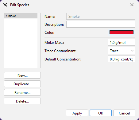
Species define the properties of contaminants in a simulation. These may be hazardous substances like smoke or harmless components of the air like water vapor (H2O). Species that appear in the Object tree may be introduced during simulation with Sources and Sinks.
To create, modify, and delete species, you can use the Edit Species dialog. To open the Edit Species dialog, on the Model menu, click Edit Species or double-click on Species in the Object tree. The figure in Figure 55 shows the dialog being used to edit a species.
Sources and Sinks introduce or remove contaminants in Zones during a simulation.
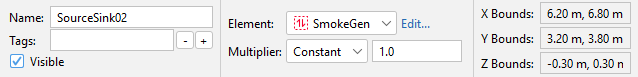
As in Figure 56, properties include
Sources and sinks are both created by the Source/Sink tool in the Workspace.
Source/Sink Elements define the model used to generate and remove contaminants at a Source/Sink (Sources and Sinks). Each source/sink must specify a source/sink element and individual source/sink elements can be used by multiple source/sinks.
To create, modify, and delete source/sink elements, you can use the Edit Source/Sink Elements dialog. To open the Edit Source/Sink Elements dialog, on the Model menu, click Edit Source/Sink Elements. The dialog in Figure 57 shows the dialog being used to edit a source/sink element.
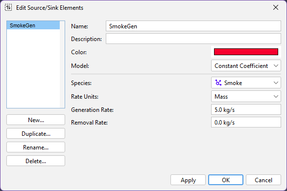
CONTAM provides a number of models for modeling generation and removal rates of contaminants. Depending on the model, a Source/Sink may act as either a source, a sink, or both.
Only the Constant Coefficient model is available in Ventus; transient contaminant generation and removal can be scheduled via the Properties panel for each instance of Sources / Sinks.
This model generates or removes contaminants at a constant mass rate.
The parameters for creating a source/sink element using the Constant Coefficient model are:
Once Source / Sink Elements are defined, the Source/Sink tool (![]() ) can be used to place Sources and Sinks in order to add or remove contaminants from the Zones they are attached to.
) can be used to place Sources and Sinks in order to add or remove contaminants from the Zones they are attached to.
Remember, Sources and Sinks add or remove contaminants from the Zones they are attached to. These contaminants may or may not impact the air density of the attached Zone, depending on whether the Species' Parameters declare Trace or Non-trace status.
Weather and Wind properties could be accessed by selecting Weather and Wind on the Model menu. Specified values can be set for each of several Scenarios, but each Scenario maintains Steady State Weather Data.
The relative humidity as a fraction, between 0.0 and 1.0.
Wind Profiles are used to combine a wind induced pressure condition with the indoor air pressure to calculate wind pressure for assigned Flow Paths. Typically, wind profiles are associated with exterior Flow Paths that connect with ambient conditions. They work by defining a relationship between the average wind pressure coefficient for the face of a building and the angle of incidence of the wind on the face of the building.
Simple Air Handling Systems (Simple AHS) provide a way to define air handling systems for the addition or removal of gasses (mass) from a model.
Each AHS Zone Point Supply or Return point must specify a Simple AHS.
Ventus provides a <global> AHS by default.
To create, modify, or delete Air Handling Systems, you can use the Edit Air Handling Systems dialog. To open the Edit Air Handling Systems dialog, on the Model menu, click Edit Air Handling Systems. The dialog in Figure 58 shows the dialog being used to edit a Flow Path element.
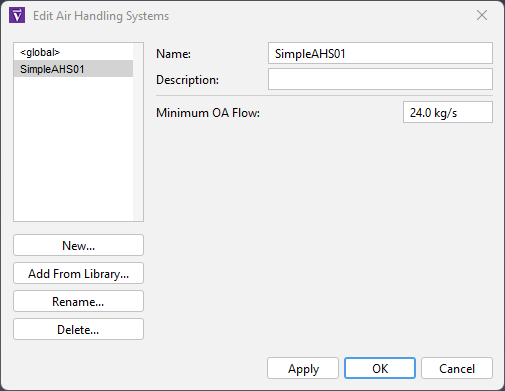
Minimum OA Flow value is overwritten. See Known Issues.
Custom AHS definitions can be saved to a Ventus library file (file extension .vlib).
Multiple Zone Supply and Return points can be specified in Zones to add or remove gasses (mass) to/from the Zones they are placed in. The result of this positive or negative mass flow will force flow through connected Flow Paths.
The following properties are available on the Properties panel for each AHS Zone point:
Supplies and Returns are both created using the AHS Zone Point tool (![]() ) in the workspace.
) in the workspace.
Ventus runs simulations using the ContamX software maintained by NIST.
This software is included with Ventus and can be found in the installation folder (e.g., C:\Program Files\Ventus 2024\contam-x-3.4.0-win64 ).
When running a simulation, a PRJ input file is created and the simulator executable is invoked on the input file similar to how it might be run for the command line.
When the simulation is finished, Ventus automatically collects and displays output for analysis. Remember, Ventus helps with results analysis by making a number of files associated the simulation more accessible (see Processing Results).
Some options that impact the entire simulation rather than specific elements like Flow Paths and zones can be controlled using the Simulation Parameters dialog.
To edit or review simulation parameters: on the Analysis menu, select Simulation Parameters.
0 s and 86,400 s (24 h).1 s and 86,400 s (24 h).When the simulation is launched, the Run Simulation dialog will appear. This dialog displays scrolling text associated with running the executables responsible for performing the simulation.
Typically, a simulation will contain output from two commands: one for contamx.exe which is the simulator and one for prjread.exe which is used to convert the SIM binary output file to human-readable output that will be collected by Ventus.
Ventus helps with results analysis by making a data associated the simulation easily accessible. After a simulation, the data derived from these files is available in the following user interface locations:
Additionally, the results files are populated inside simulation folder(s) in the same directory as the Ventus model.
After running a simulation, results data is added to the Object Tree for viewing and analysis. All output data is available for viewing as text output data.
id of interest (e.g., getting started).Link Flows (LFR)).When finished, you can close the browser window and reopen at any time. The temporary file displayed by the browser will be deleted when Ventus exits.
Any results data appearing in the Object Tree has been integrated with the Ventus data model and will be saved with the VNTS file; it is not necessary to keep any simulation files other than the VNTS file when sharing or archiving simulation data.
The following list describes each of the Object tree results files:
In the file paths above, id is the scenario identifier.
For single scenario simulations, this identifier will match the VNTS filename.
For multiple scenario simulations, all scenarios will be added to the Object panel and their identifiers will additionally include a text representation of the scenario parameter values used to generate the input for that simulation.
After running a Transient simulation, time controls will be shown below the 2D/3D workspace. These controls can be used to animate flow vectors in the 2D/3D workspace and to filter tables in the Results Panel.
To begin animation playback, press the play button ![]() at the bottom of the Workspace.
As the animation is playing, the time slider will move, and the animation can be paused
at the bottom of the Workspace.
As the animation is playing, the time slider will move, and the animation can be paused ![]() .
The buttons
.
The buttons ![]() and
and ![]() will move the time slider to the beginning and end, respectively.
The buttons
will move the time slider to the beginning and end, respectively.
The buttons ![]() and
and ![]() will slow down and speed up the animation by factors of two.
The time field can be used to go to a specific timestep.
will slow down and speed up the animation by factors of two.
The time field can be used to go to a specific timestep.

The status bar at the bottom of the Ventus window shows information about playback status, as in Figure 60
minutes:seconds.
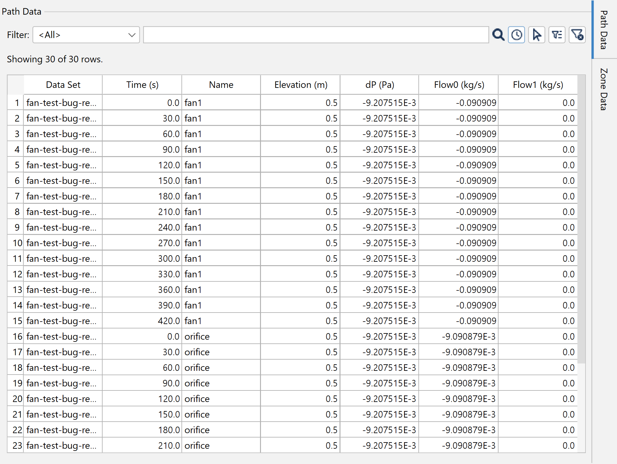
Ventus uses the SQLITE3 simulation output data to identify pressure change (dP ![]() ) and flow volume (Flow0
) and flow volume (Flow0 ![]() ) data associated with each Flow Path.
This data is in the Path Data results subtree and appears in the Workspace as colored vectors rooted at the corresponding Flow Path.
) data associated with each Flow Path.
This data is in the Path Data results subtree and appears in the Workspace as colored vectors rooted at the corresponding Flow Path.
The direction of vectors displayed in the Workspace is determined by the direction of positive flow for the Flow Path (see Flow Path Properties) and the sign of the output data. For example, if a pressure difference vector is positive and the Flow Path indicates that the direction of positive flow is from Zone A to ambient, that vector will extend from the Flow Path into the ambient Zone. If the pressure difference vector is negative, the vector will be drawn extending into Zone A.
The position of the vector origin for single-point Flow Paths is the location of the Flow Path. In situations where a Flow Path connects two zones across a gap, the vector will be drawn originating from the Flow Path point attached to the Zone in the direction of the vector.
The length of vectors displayed in the Workspace is proportional to the vector with the greatest magnitude in that simulation. Lengths for pressure differences and flow rates are calculated independently.
When viewing results data, the Flow Paths themselves can sometimes obscure or crowd path data vectors, and it can be helpful to hide them.
To hide Flow Paths: in the Object Tree, right-click Flow Paths and select Hide, or use the Show Flow Paths view tool described in Render Options.
To restore Flow Path visibility: in the Object Tree, right-click Flow Paths and select Show (or use the Show Flow Paths view tool). If this shows all Flow Paths and not just those in the current active level, toggle the level selection box to restore the level visibility filter.
Ventus also provides results info for selected objects in the Quick Reference data panel, just beneath the workspace and the Results Timeline. Results information is only displayed in this location for selected Zones, Flow Paths, and results vectors when results data associated with those objects is available; otherwise information associated with the current tool is shown.
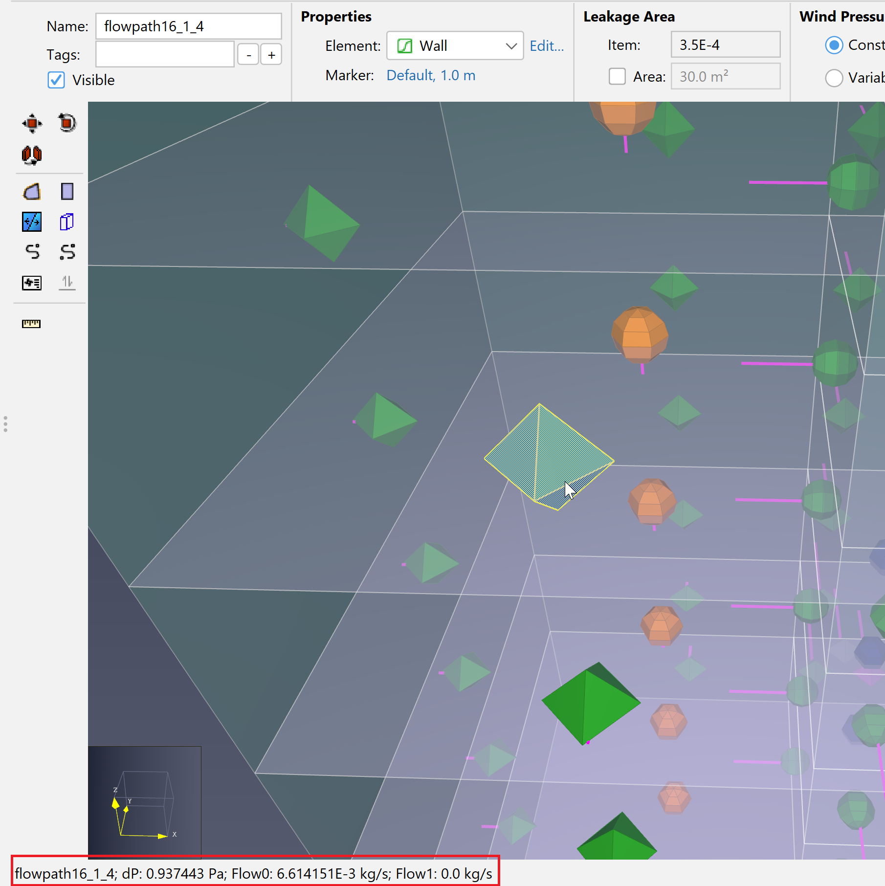
The Results Panel provides an in application display of Ventus run results along with tools to filter and isolate specific results of interest.
The Path Data tab shows data from each of the Link Flows (LFR) result sets. The following filters may be used to limit the displayed data for performing an analysis of a shaft or other isolated group of results.
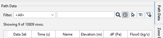
The Zone Data tab shows data from a combination of the Node Flows (NFR) and Node Concentrations (NCR) result sets. The following filters may be used to limit the displayed data for performing an analysis of an isolated group of results.
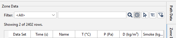
The 2D Plot dialog (Figure 64) provides a graph of Transient simulation results.
When opening the 2D Plot dialog from a context menu, plots related to the selected objects will be automatically selected.
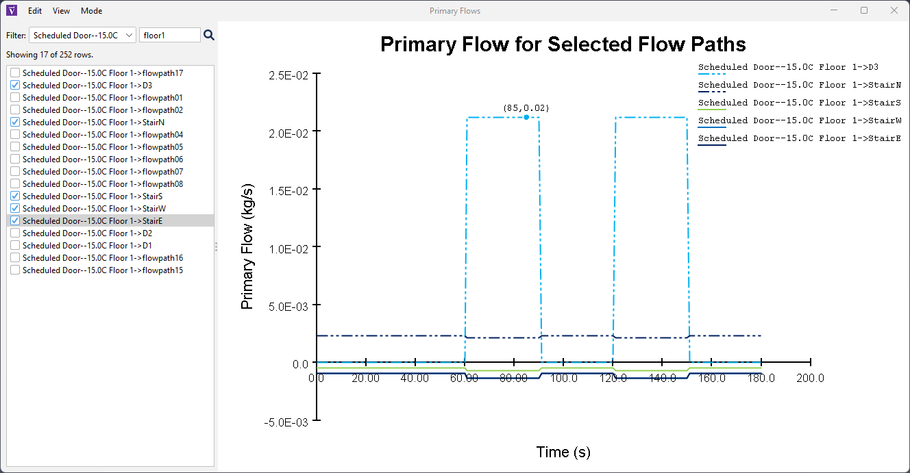
On the left side of the 2D Plot dialog a list of Flow Paths or zones is shown. Each Flow Path or Zone in this list may appear once per data set in the results. The names of these objects are annotated with the data set and group name. These annotations can be hidden by unchecking Show Group Names or Show Data Set in the View menu of the 2D Plot dialog.
You may add or remove a plot by checking or unchecking the objects in this list.
Plots which were previously selected in this list will remain visible even while using these filters.
The 2D Plot dialog provides several quantities to plot. You may select which quantity to plot when opening the dialog or from the Mode menu in the dialog.
Since the simulation run has completed, the Results data has been captured in the VNTS file.
Thus, a Ventus file can be shared which includes all the relevant geometry and results.
Copies of the results data are still available in the folder location, as well.
The results folder(s) will have an identifier similar to ID.
<id>-20.0C and <id>-10.0C).For the default conversion of air in CONTAM modeling software, a pressure of 101.325 kPa and a temperature of 20 °C is assumed. 0.0 % RH is also assumed, leading to the density of 1.20410 kg/m3.
Some options can only be activated using program arguments or environment variables. These options are associated with uncommon workflows such as troubleshooting or testing experimental features. Any saved data associated with experimental features may not be retained in future versions.
For example, if an environment variable and a program argument are both specified, the program argument will be used, and the environment variable will be ignored.
| Maximize compatibility of graphics settings. Can be used to reset preferences when a graphics configuration preference prevents the software from running. Disabled preferences will remain disabled in future non-safemode runs until manually re-enabled. | ||
| Startup Parameter | Enivronment Variable | PROPS File Entry |
-DSafeMode | ||
This option accepts no additional parameters.
Start the software in safe mode: graphics preferences will be reset to maximize compatibility. | ||
| Pass parameters to the Java VM prior to launching the software. | ||
| Startup Parameter | Enivronment Variable | PROPS File Entry |
-J[arg] | ||
Parameter [arg] will be passed directly to the JavaVM on startup prior to launching the application.
Passes the parameter | ||
Override automatic locale selection and use preset values for user.language and
user.country. Controls selection of localization bundle. | ||
| Startup Parameter | Enivronment Variable | PROPS File Entry |
| ||
Parameter
Start the software with the specified user.language (en: English).
Start the software with the specified | ||
| Add ContamW PRJ export option to the file menu. Exported PRJ file will not contain sketchpad data and will not open in ContamW. Suitable for using DIFF tooling to compare with ContamW-generated files than the annotated simulation PRJ file generated by Ventus. | ||
| Startup Parameter | Enivronment Variable | PROPS File Entry |
| -J-Dexport_prj_enable=[value] | VNTS_EXPORT_PRJ_ENABLE=[value] | ventus.export.prj.enable=[value] |
Parameter
Enable PRJ comparison export. | ||
The following sections provide solutions to common troubleshooting problems
For troubleshooting tips on licensing Issues, see our Licensing FAQs.
Ventus utilizes many advanced graphics card features in order to provide accelerated and enhanced display of models.
Sometimes these graphics features combined with certain display drivers can cause display issues or crashes on startup. The first step in these cases is to ensure you have the latest operating system updates and graphics drivers installed. If you do, and you still have display problems or crashing on startup, you can start Ventus in Safe Mode, which disables several graphics features.
To start in Safe Mode:
cmd.
Then press Enter.cd "C:\Program Files\Ventus 2025".ventus -DSafeMode.If you encounter display problems or crashes, please let us know the make/model of your video card and what video driver you are using, even if Safe Mode fixes your issues. That will help us improve the software in future updates.
When running large models, it is possible that an out of memory error will be encountered. If this occurs, you can increase the default Java heap size. In our experience, the maximum size can be specified to approximately 70% of physical memory. By default, Ventus will specify a java heap size of 50% of physical memory.
To specify the memory, you can either run from a command line or change the Start Menu shortcut properties.
To run from a command line, open a command window and then go to the Ventus installation directory (usually C:\Program Files\Ventus 2025).
Execute Ventus on the command line using the -J-Xmx argument.
In this argument, the -J specifies that the command will be passed along to the Java VM, not Ventus.
For example, ventus -J-Xmx1200m will request 1200 MB of memory.
To edit the Ventus shortcut properties
. Right-click on the Ventus icon
. Select the Shortcut tab
. Edit the Target by adding a space and -J-Xmx1200m to the end of the Target.
A typical Target will then read C:\Program Files\Ventus 2025\ventus.exe" -J-Xmx1200m.
Dols, W. Stuart, and Brian J. Polidoro. 2020. NIST Technical Note 1887, CONTAM User Guide and Program Documentation, Version 3.4. Revision 1. National Institute of Standards and Technology, Gaithersburg, Maryland, USA: NIST.