 |  |
 |  |
 | |
General usage information for the Pathfinder Results Viewer
There is a newer version of this document. To view the latest version, click here.
Thunderhead Engineering makes no warranty, expressed or implied, to users of this software, and accepts no responsibility for its use. Users of this software assume sole responsibility under Federal law for determining the appropriateness of its use in any particular application; for any conclusions drawn from the results of its use; and for any actions taken or not taken as a result of analyses performed using these tools.
This software is intended only to supplement the informed judgment of the qualified user. The software package is a computer model that may or may not have predictive capability when applied to a specific set of factual circumstances. Lack of accurate predictions by the model could lead to erroneous conclusions. All results should be evaluated by an informed user.
All other product or company names that are mentioned in this publication are tradenames, trademarks, or registered trademarks of their respective owners.
This guide tells you how to use the results visualization software that accompanies Pathfinder. It assumes a basic understanding of the work flow when using these platforms to model fire and movement. For introductory guides PyroSim and Pathfinder, refer to the support materials for each product online at https://support.thunderheadeng.com/
This guide is the primary source of documentation for the Results visualization software and describes how to perform common tasks. For additional information describing how different parts of the software work, refer to Technical Reference.
For documentation on other Thunderhead Engineering applications, refer to the product-specific support materials online at https://www.thunderheadeng.com
If you need assistance, or wish to provide feedback about any of our products, contact support@thunderheadeng.com
The results visualization software will be installed automatically with Pathfinder. There is no need to download or install a separate application. For more information about installing PyroSim and Pathfinder, refer to the support materials for each product online at https://www.thunderheadeng.com
Table 1 lists system requirements necessary to run results visualization.
| Operating System | Microsoft Windows 7 or newer Desktop Experience and Media Feature Pack are required due to a dependency on Windows Media Player (wmvcore.dll). |
| Memory | 4 GB (required) |
| Display Adapter | Support for OpenGL 1.2 (required) |
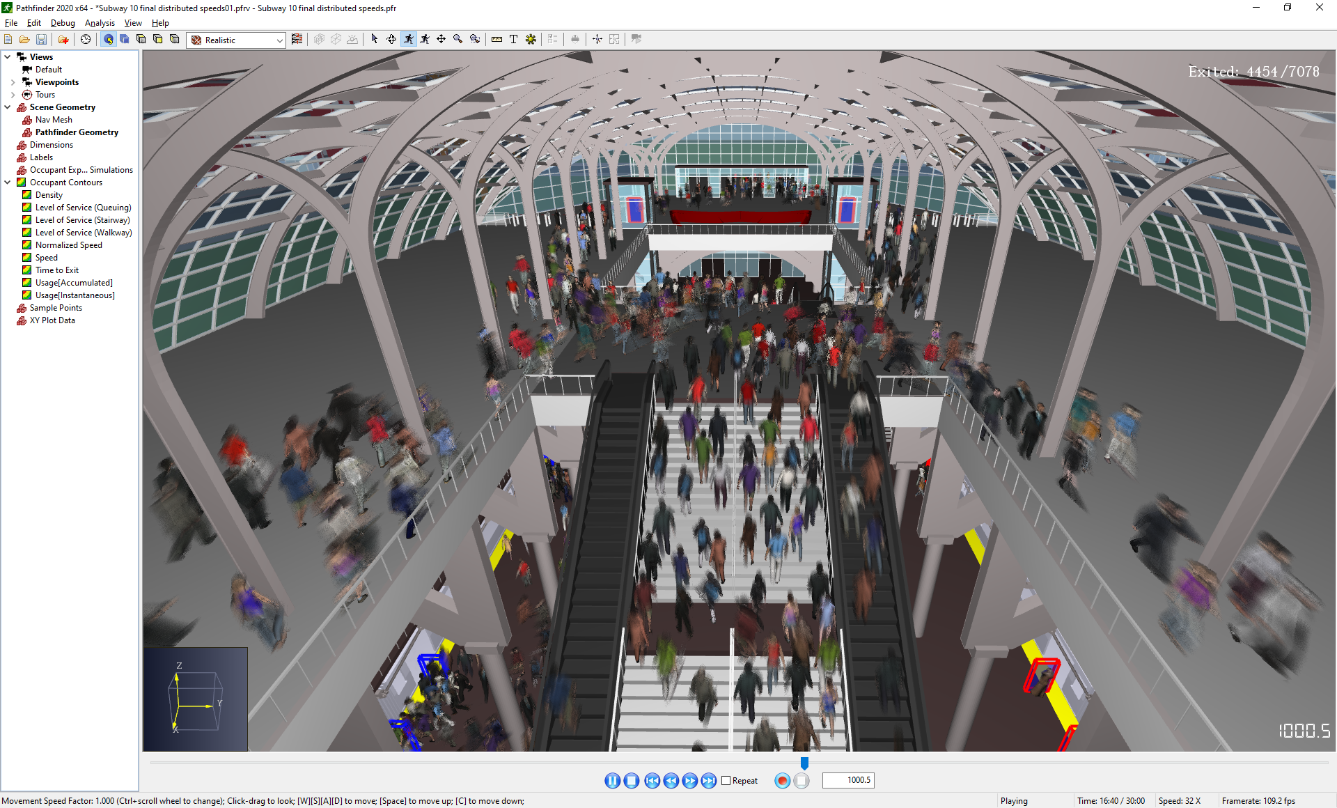
Results visualization performance (measured in frames per second, or FPS) is controlled by the number of occupants in the model, the complexity of the geometry, and the resolutions of the FDS solution meshes. In one Pathfinder experiment, a single-room model containing 3,000 occupants and 4 geometry triangles operated at 15 FPS. By comparison, a complex model with 50,000 occupants and 1,300,000 geometry triangles operated at 5 FPS.
Performance can be improved in several ways:
Results visualization requires a PyroSim or Pathfinder license. Additional information on license activation is located on the corresponding software download page.
To locate a license, a search is performed in standard locations for a valid license. In addition, license locations listed in the PROPS files for PyroSim and Pathfinder are searched.
The search order is shown below:
Results.props or -rlmpath argument.%PROGRAMDATA%\Application Data\Results\license%APPDATA%\Pathfinder\Pathfinder.props%PROGRAMDATA%\Pathfinder\license%APPDATA%\PyroSim\PyroSim.props%PROGRAMDATA%\PyroSim\licenseResults will operate if any valid license is found.
It is recommended to run PyroSim or Pathfinder before running the results software to ensure a valid license location is present in the corresponding PROPS file.
For advanced use and license troubleshooting, two command-line options are available:
-rlmpath <path> | Specify a custom RLM license location. This location will be prepended to the list of license search locations. To add a local license folder to the search path:
To add a floating license server to the search path (port@computer):
Results will save the value of |
-rlmstrict | Prevent results from appending default search locations to the RLM license search path. When this option is set, only the custom path and the executable folder will be searched for licenses. To use only the executable folder and (optionally) a license path stored in the PROPS file entry
To use this option in combination with
|
The Results application can be used to visualize results from PyroSim/FDS and Pathfinder. It operates much like a video player in that it allows users to play, pause, stop, slide, and speed up and down time. It is completely 3D and allows users to navigate through a model.

There are several per-user settings that control how the Results application works.
Many of these global settings can be found in the Preferences dialog, which can be opened by clicking the File menu and selecting Preferences.
These preferences are stored in a PROPS file called Results.props.
By default, this file can be found in: %APPDATA%\Pathfinder\Results.props
The PROPS file is stored in a plaintext format and can be viewed or edited with any conventional text editor.
The Results application allows users to create, save, and load results visualizations. A results visualization is a collection of settings that define which Pathfinder and FDS results are to be loaded and how those results are to be displayed. It also contains information entered by the user, such as views, tours, colorbar settings, time settings, annotations, object visibility, etc.
Results visualization files end with either .pfrv when saved from Pathfinder Results or .smvv when saved from PyroSim Results.
When Pathfinder or FDS results are viewed for the first time, a results visualization is automatically created and saved containing the results data. The visualization file name will match that of the originating PTH or PSM file. If a visualization file already exists with a matching name, the existing visualization is loaded instead. The same behavior is used when double-clicking a PFR or SMV file in Windows explorer.
To create a new, empty visualization, on the File menu click New Results Visualization ![]() or press Ctrl+N on the keyboard.
or press Ctrl+N on the keyboard.
To load results into the current visualization, see Loading Results.
To save a visualization, on the File menu, click Save Results Visualization ![]() or press Ctrl+S on the keyboard.
Alternatively, the results visualization can be saved to a new file by opening the File menu and clicking Save As.
This allows several visualizations of the same Pathfinder/FDS results to be saved, each with their own settings.
or press Ctrl+S on the keyboard.
Alternatively, the results visualization can be saved to a new file by opening the File menu and clicking Save As.
This allows several visualizations of the same Pathfinder/FDS results to be saved, each with their own settings.
To open an existing visualization, on the File menu, click Open Results Visualization ![]() or press Ctrl+O on the keyboard. When opening an existing visualization, the previously active results (e.g. fire/smoke, occupant contours, occupant paths, etc.) will be shown.
or press Ctrl+O on the keyboard. When opening an existing visualization, the previously active results (e.g. fire/smoke, occupant contours, occupant paths, etc.) will be shown.
Because this may make some visualization files take longer to load, this behavior can be disabled by opening the Preferences dialog and unchecking Show previously active results on open.
The Results application can show exactly one results data file from Pathfinder and one file from PyroSim/FDS at the same time. If results are opened that are of the same type as those already loaded, the current results of that type will be replaced with those from the new file. For instance, if Pathfinder results A are opened and then PyroSim results B, both A and B will be shown. If Pathfinder results C are then loaded, only B and C will be shown.
To load Pathfinder or FDS results into the current visualization, on the File menu, click Load Results ![]() or press Ctrl+Shift+L on the keyboard.
Choose a PFR file to open Pathfinder results or choose an SMV file to open FDS results.
or press Ctrl+Shift+L on the keyboard.
Choose a PFR file to open Pathfinder results or choose an SMV file to open FDS results.
If the PFR or SMV file was opened in a previous version of Results, there may be additional data that can be imported into the current visualization, including views, tours, unit preferences, time settings, and occupant contour settings. If the Results application detects any of this data, it will ask if that data should be imported.
Alternatively, some of this data can be imported later under the File menu by choosing Import→Import Occupant Contours or Import→Import Views.
Results can be individually unloaded as well without losing any of the associated visualization data. To do so, on the File menu click either Unload FDS Results or Unload Pathfinder Results. If another results file is loaded, the previous settings will be applied to the new results.
For instance, say Pathfinder results A is loaded, and an Average Density contour is added. If results A is then unloaded and Pathfinder results B is loaded, the Average Density contour, as well as all other contour settings are maintained and can be used with results B. The same is true if results file A is still loaded and B is loaded to replace A.
When results files are loaded into a results visualization, the paths to those files are stored relative to the visualization file’s directory if possible. This allows entire folders with results and their visualizations to be copied or moved to another location without breaking the links between files.
For instance, say a visualization file is saved to C:\case1\case1.pfrv, and it has loaded both C:\case1\pathfinder\case1_occs.pfr and C:\case1\pyrosim\case1_fire.smv.
In this case, the visualization file would have saved the paths internally as pathfinder\case1_occs.pfr and pyrosim\case1_fire.smv.
If the visualization and results need to be moved, this can be done by simply moving all the contents of the C:\case1\ folder (or the folder itself) to another location.
The same can be done with copying as long as the files are pasted to another location such that the filenames do not change.
Each results file (Pathfinder or FDS) has its own timeline.
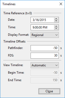
The Timelines dialog, as shown in Figure 2, can be used to control the timelines, set a reference clock time, and set the time range displayed in the results as controlled by the time slider.
To open the timelines dialog, perform one of the following:
There may be up to three timelines in the results. There is always a Global timeline, and depending on which results are loaded, there may also be a Pathfinder timeline and an FDS timeline.
The Global timeline has a Time Reference that is used to synchronize the Pathfinder and FDS results. The time reference has an associated calendar Date and a clock Time, such as June 3, 2018 at 3:47 PM. This value defaults to the date/time at which either the Pathfinder or FDS results was first created. It may be changed, however, to correspond with a real date/time either for event reconstruction or scenario planning.
The date/time may optionally be shown in the 3D View by going to the View menu and under the Time Display sub-menu, selecting either the Date/Time or Time option. The display of the date/time will automatically adjust depending on the current playback time. The Display Format defines how the date/time will be displayed.
The following formats are available:
7/3/2018 3:47:00 PM.
In Germany, however, it might display as 03.07.2018 15:47:00.ISO 8601 international standard.
In this format, the date/time will appear in all regions as 2018-07-03 15:47:00.Timeline Offsets are used to change the beginning time of the FDS and Pathfinder results relative to the global time reference in order to synchronize the timelines properly. This is necessitated by the fact that Pathfinder and FDS simulations are often run as though the beginning time is at some arbitrary value, usually t=0. When loading both Pathfinder and PyroSim/FDS results together at the same time, however, the results files might need to be offset from one another.
The View Timeline specifies the global time range displayed in the results.
It can be one of these values:
To demonstrate the timeline parameters, suppose a hypothetical fire and evacuation scenario is recreated in PyroSim and Pathfinder.
The fire is simulated such that the fire starts immediately at t=0. The Pathfinder simulation is also simulated with the evacuation taking place at t=0.
If both these results files were to be loaded with no changes to the timelines, the occupants would leave as soon as the fire started. In order to synchronize the results properly, the date, March 23, 2003 at 3:00 PM is entered for the reference time. The FDS time offset is set to -120 s to represent that the fire started 2 minutes earlier. The Pathfinder time offset is set to 180 s to represent the 3 minutes of pre-movement time. Now when played back, the results will be synchronized properly and show the correct date/time in the 3D View.
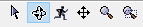
Once a model is loaded, the navigation tools (Figure 3) work similarly to those found in Pathfinder.
At any time, press Ctrl+R to reset the camera view or in the View menu click Reset Camera.
There are two main cameras that can be used to view the model. When switching between cameras, the Results application tries to maintain the same viewpoint if possible.
Either camera can be reset to several pre-defined viewpoints by selecting the appropriate toolbar button (Figure 4). These viewpoints include the Top, Front, and left Side (highlighted in red).

Views can be used to store and retrieve various view state in the Results and to create animated tours of the model. For more information on using and creating views and tours, see Views, Tours and Clipping.
There are several geometry sets that may be available with Pathfinder and PyroSim/FDS results. When results are loaded, the available geometry sets are shown under the Scene Geometry group of the Navigation View.
By default, with the exception of the Pathfinder Navigation Mesh and Background Images, only one geometry set may be shown at a time. This can be changed in the Preferences dialog, by unchecking Scene Geometry→Only show one at a time. To go to the Preferences dialog, in the File menu select Preferences.
To switch between the geometry sets, either double-click the desired geometry set in the Navigation View or right-click it and select Show. The labels for geometry sets that are active become bold in the Navigation View.
The following geometry sets may be available for Pathfinder results:
The following geometry sets may be available for PyroSim/FDS results:
The default geometry set shown in the results depends on which results type (Pathfinder or FDS) was loaded first and which geometry sets are available. For the results type that is loaded first, the geometry is chosen by selecting the first available set as listed above for each type.
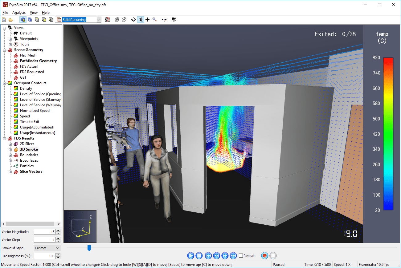
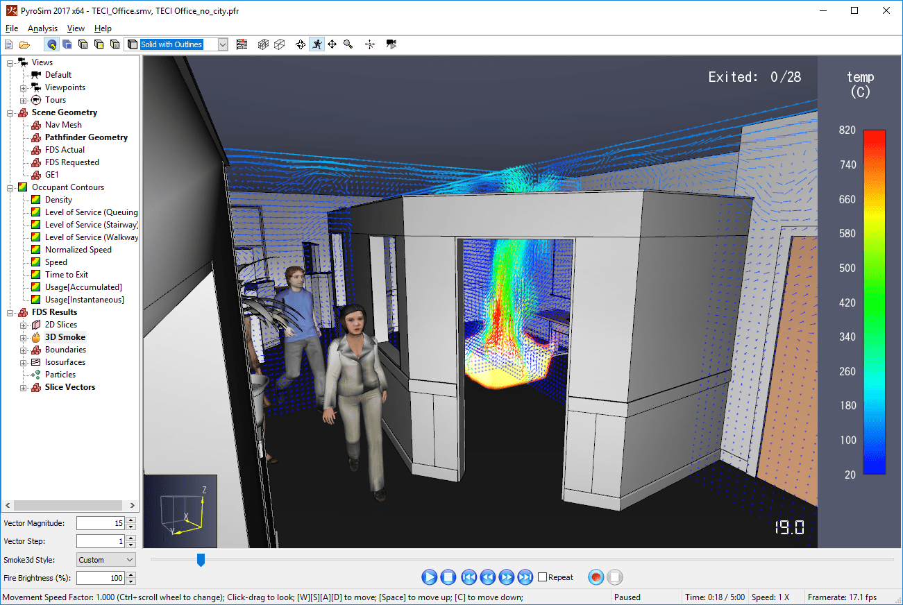
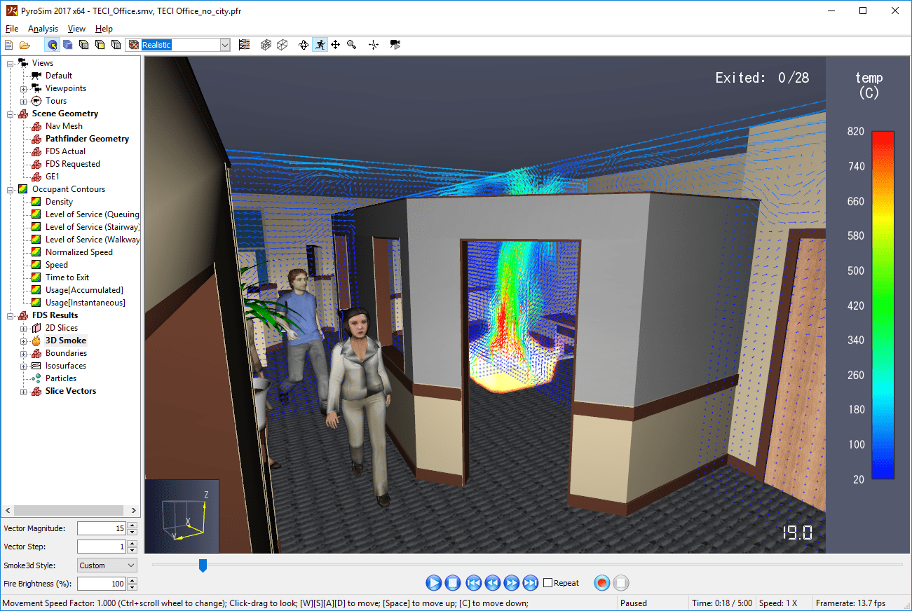
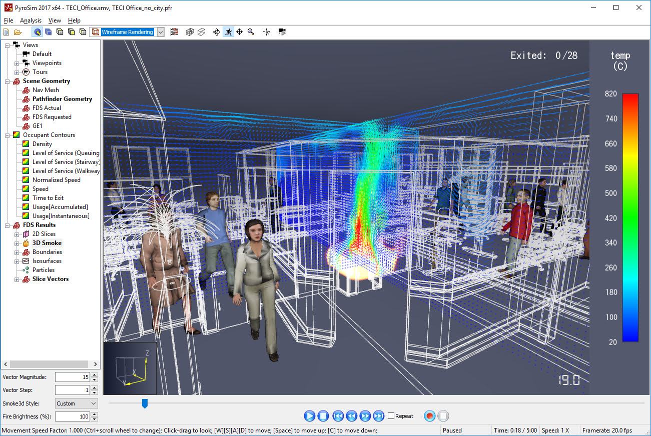
With the exception of the Nav Mesh, geometry data can be shown in several different modes. To change the mode, click the mode drop-down box in the main toolbar (Figure 5).

The following modes are available:
| |
| |
| |
Objects in the Results can be selected by clicking them in either the 3D View or Navigation View. Selection is synchronized in all the views, which means that if you select an object in one view, it will also be selected in the other views. To select multiple objects, on the keyboard hold Ctrl while clicking the objects. To clear the selection, press Esc or click in empty space in one of the views. Alternately, on the Edit menu, click Clear Selection.
When an object is selected, the name of the object will be displayed in the status bar at the bottom of the screen. In addition, the object will be highlighted in all the views.
Some objects have additional actions that can be performed on them once they are selected. Right-click on the selected objects or right-click an unselected object to select it and show a context menu with additional actions.
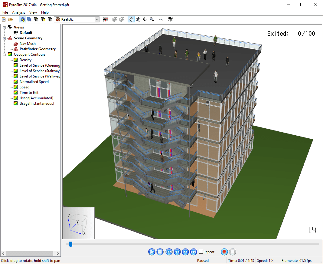
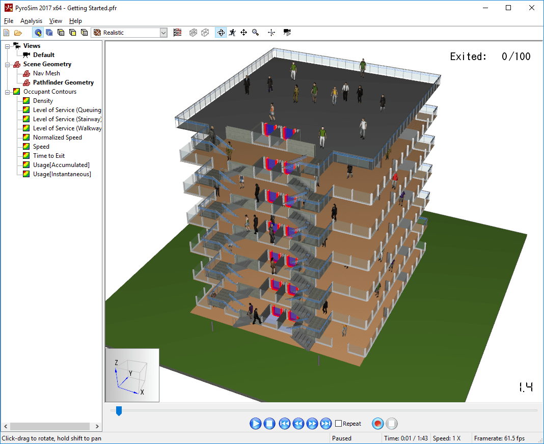
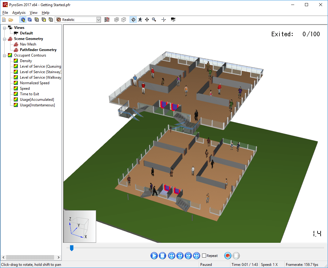
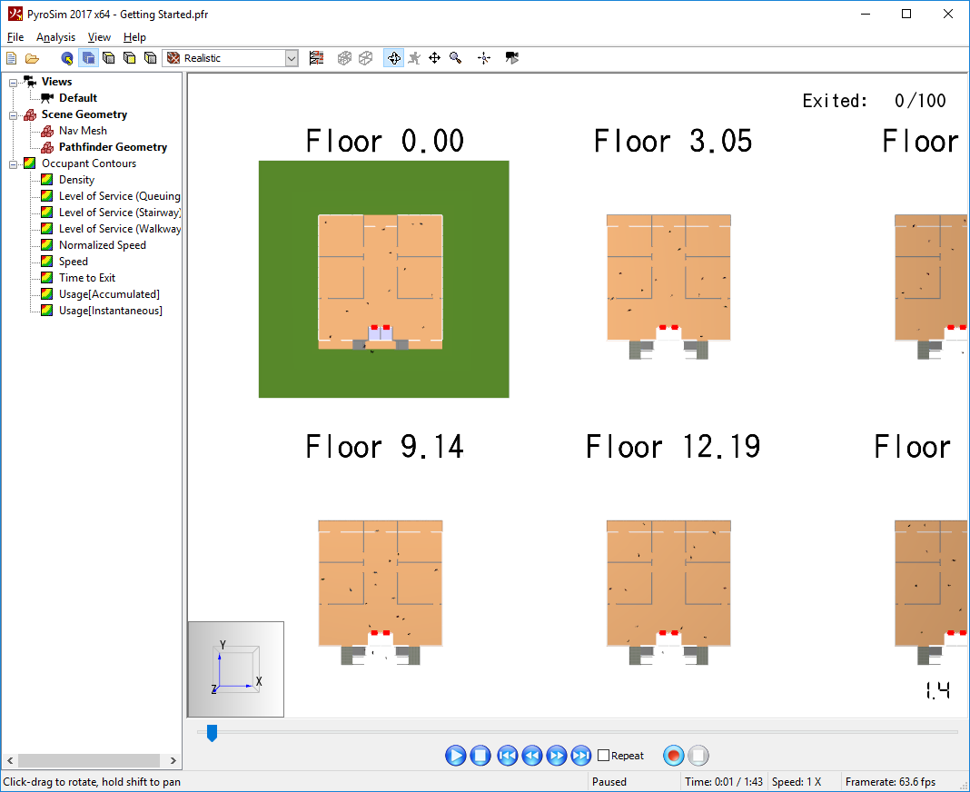
Some models are composed of several floors, causing each floor to obscure the one below it as shown in Figure 11. The Results application provides a variety of options for viewing the model such that building contents can be easily observed. One option is to view the model with the floors stacked vertically but separated by a settable distance. Another option is to view the model with the floors lying in the XY plane so that they can all be viewed from overhead. Both options allow a wall clip-height to be specified and for certain floors to be selectively shown or hidden.
 |  |
 |  |
To use any of the layout options, floors must first be defined. If the floors were defined in Pathfinder or PyroSim, they will carry through to the 3D visualization and no additional input is needed.
If they have not been defined or they need to be modified, this can be done as follows:
 | 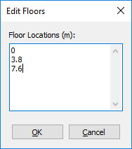 |
The Results application will partition the geometry among the floors such that the bottom floor contains all geometry from \(-{\infty}\) to the next floor’s location, the top floor contains all geometry from its location to \(+{\infty}\), and every other floor contains geometry from its location to the next floor’s location.
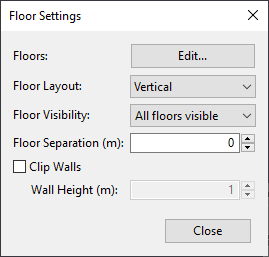
Once floors are defined, there are several ways to lay out the floors and clip the walls, which can all be done from the Floor Settings dialog. The Floor Layout controls how the floors are laid out in the view.
The following options are available:
In addition to showing and hiding floors in the Edit Floor Settings dialog, floors can also be isolated based on a selection. To do so, select the desired objects whose floors you want to isolate. Then right click and choose Show Floors for Selection. This will only show the floors containing the selected objects.
The floors are chosen as follows:
To easily show all the floors again, either right-click on empty space in the scene view and choose Show All Floors or in the in the View menu, choose Show All Floors. The floors can also be shown again using the Floor Settings dialog.
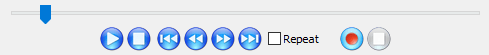
To begin animation playback, press the play button ![]() at the bottom of the 3D View.
As the animation is playing, the time slider will move, and the animation can be paused
at the bottom of the 3D View.
As the animation is playing, the time slider will move, and the animation can be paused ![]() .
The buttons
.
The buttons ![]() and
and ![]() will move the time slider to the beginning and end, respectively.
The buttons
will move the time slider to the beginning and end, respectively.
The buttons ![]() and
and ![]() will slow down and speed up the animation by factors of two.
In addition, the playback can be looped by checking the Repeat button.
will slow down and speed up the animation by factors of two.
In addition, the playback can be looped by checking the Repeat button.
The status bar at the bottom of the screen shows information about the current navigation tool and about playback status.
Results can be viewed as a simulation is running, but they will only show the amount of time available at the last load or refresh. To refresh the results at any time, press F5 on the keyboard or select Refresh Results in the File menu. The current playback time will be restored after refreshing the results, making the refresh as seamless as possible. If the results are launched from Pathfinder before the simulation is finished, the Results application will automatically refresh and come to the front of the screen when the simulation completes.
The Results application streams files from disk rather than loading the entire results files into memory. File streaming allows results to load quickly and enables very large results to be loaded even if there is limited system memory.
In order for file streaming to work well, the hard drive that contains the results data needs to be fast enough to load the results data at the desired playback speed. With some very large FDS results, however, even a fast disk may not be fast enough to stream the data.
These models may cause the results to stutter or pause intermittently during playback or when moving the time slider. In these extreme cases, the results can be loaded into memory.
To do so:
There are several options controlling the drawing quality and speed in the Results application, including level-of-detail rendering, hardware versus software rendering, and vertex buffers. Almost all of the options are chosen automatically depending on the capabilities reported by the graphics adapter (GPU).
To view the rendering options, in the File menu select Preferences. This will open the Preferences dialog. Next select the Rendering tab. At any time, the Max Quality button may be pressed to load settings that will give the highest quality image available, which are automatically loaded by default.
There are some cases where these settings can be problematic for the graphics adapter and can produce incorrect renderings, such as black geometry, incorrect fire, etc. If this is the case, pressing the Max Compatibility button will load settings that should work even on these problematic GPUs, at the expense of rendering quality and speed.
The following rendering options are available:
Enables shadowing in areas where light is less likely to reach, such as under objects, in corners, etc. This option generally produces more realistic and pleasing scenes, but it may have a large impact on rendering speed, depending on the system’s GPU. By default the option is off, but can be turned on manually or by selecting Max Quality.
 |  |
Uses an algorithm similar to that used in Smokeview and the compatibility renderer where many slices are drawn through a 3D dataset (Figure 22). It also has the same limitations as the compatibility renderer except that it is generally much faster for static viewpoints. This technique also does not require 3D textures, which improves its compatibility with older GPUs, but the slices are only drawn through the data at fixed angles. This becomes more visible as the camera is rotated around the scene and can produce slight, sudden shifts in the rendering.
 |  |  |
This option is only available when using the hardware shaders algorithm. It reduces banding artifacts that may be visible when the ray-marching sampling frequency is too low for the fire data as seen in the images below. It counters the banding effect by using a dithering pattern that is generally more visually pleasing. It negatively impacts the rendering speed very slightly, but is still much faster than the alternative, which is to increase the Sampling Factor.
 |  |
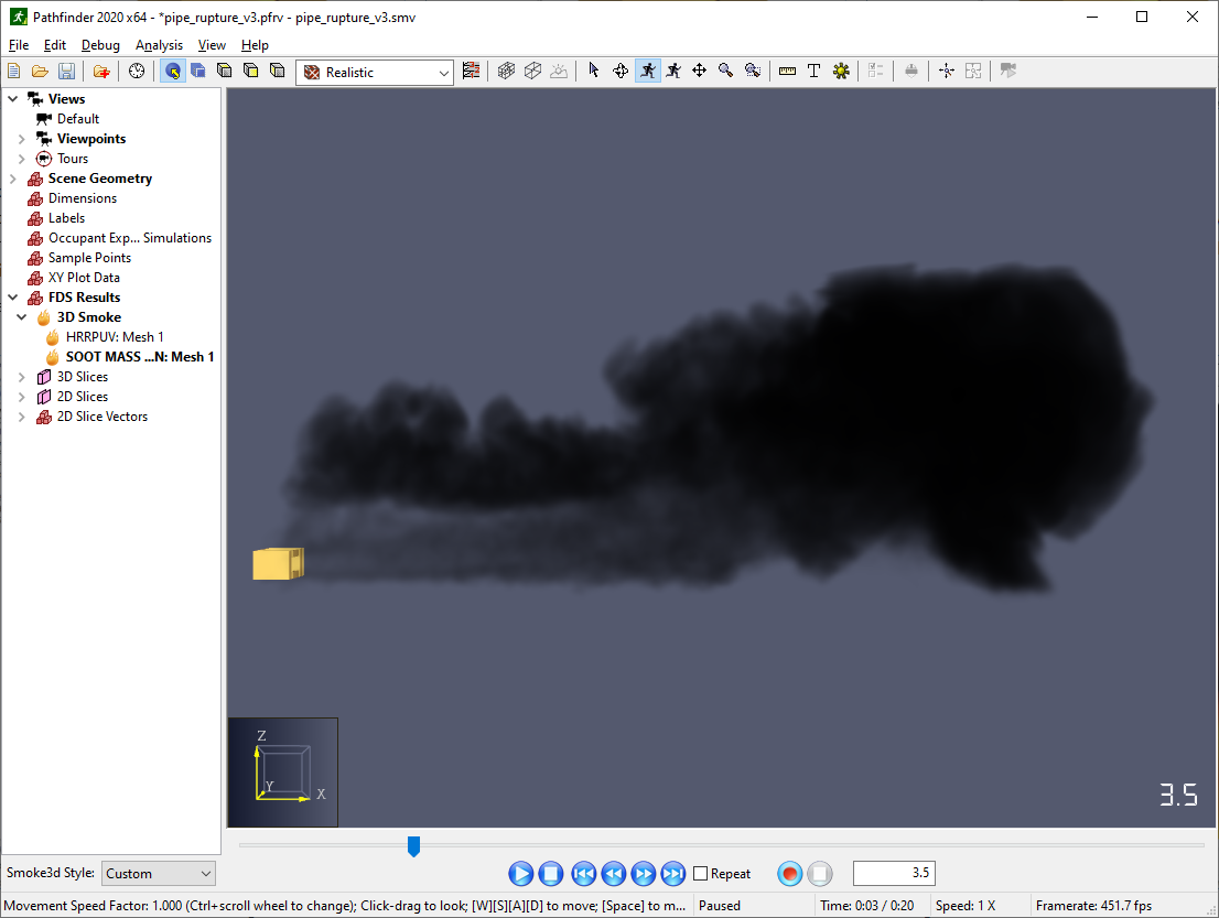
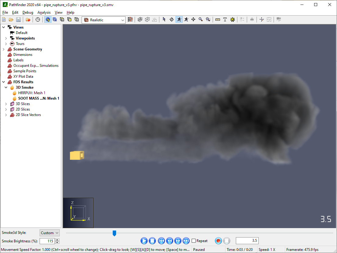
This experimental option is only available when using the hardware shaders algorithm. It simulates ambient lighting in smoke, which may help to better visualize the structure of the smoke and enhance realism as seen in the images below. This option may have a large impact on rendering speed, depending on the system’s GPU. By default the option is off, but can be turned on manually or by selecting Max Quality. When this option is enabled, an extra Smoke Brightness setting is available in the Smoke3D Properties dialog as discussed in 3D Smoke and Fire and in the Quick Settings.
 |  |
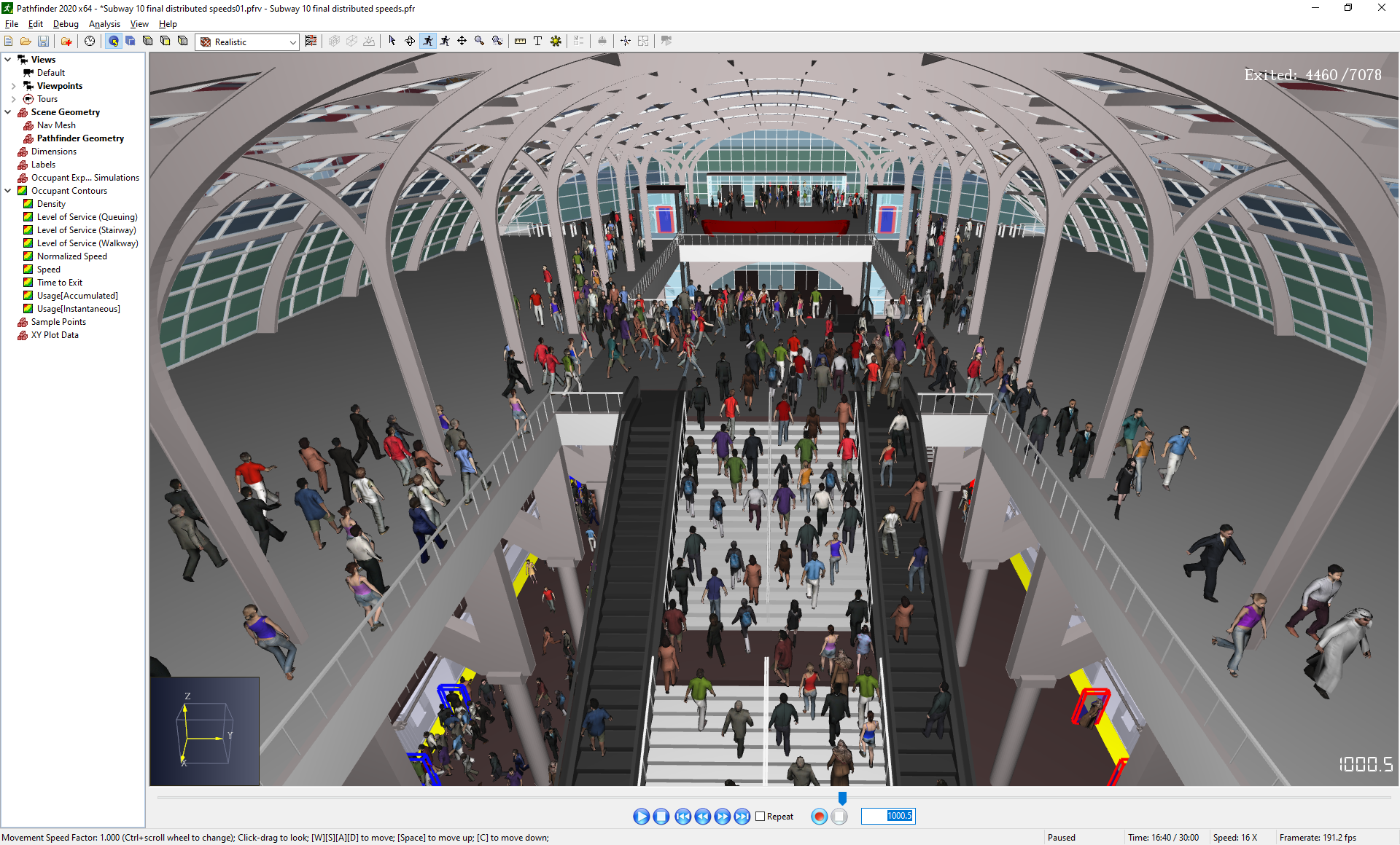
Motion blur is a graphics effect used to emulate the streaking of fast-moving objects in cinema, caused by the limited shutter speed of a motion camera. This effect is most noticable when there is fast motion on the screen such as watching a sped-up playback of Pathfinder occupants or fast movements of the camera. On the View menu, click Enable Motion Blur to enable the effect. This setting is saved with the visualization file. The images below compare a scene with motion blur enabled and disabled and were taken while playing back Pathfinder results at 16x speed.
 |  |
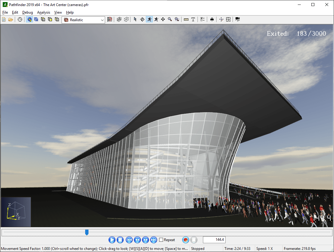
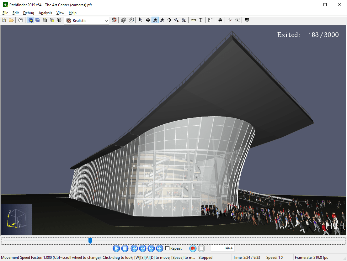
One way to improve the visual appeal of a scene, especially if it is an outdoor area or has windows to the outside, is to add a skybox. A skybox is a specialized background with more interesting features, such as sky, clouds, the sun, mountains, cityscape, etc. It is simply an image or collection of images that are displayed as if they are infinitely far away.
These images are often generated from the real world using a 360° camera or generated with CG. The features of the background completely enclose the scene such that when the scene camera is rotated, the background rotates as well but if the camera moves, the skybox stays in place.
The Results application allows a skybox to be easily added to the scene for added visual appeal.
An example skybox is shown in Figure 29:
 |  |
To add a skybox, in the View menu, click Edit Skybox. This will open the Edit Skybox Dialog as shown in Figure 31.
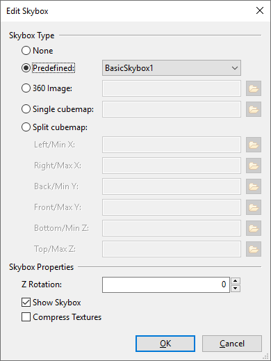
The following options are available for specifying a skybox:
These images look similar to the following:
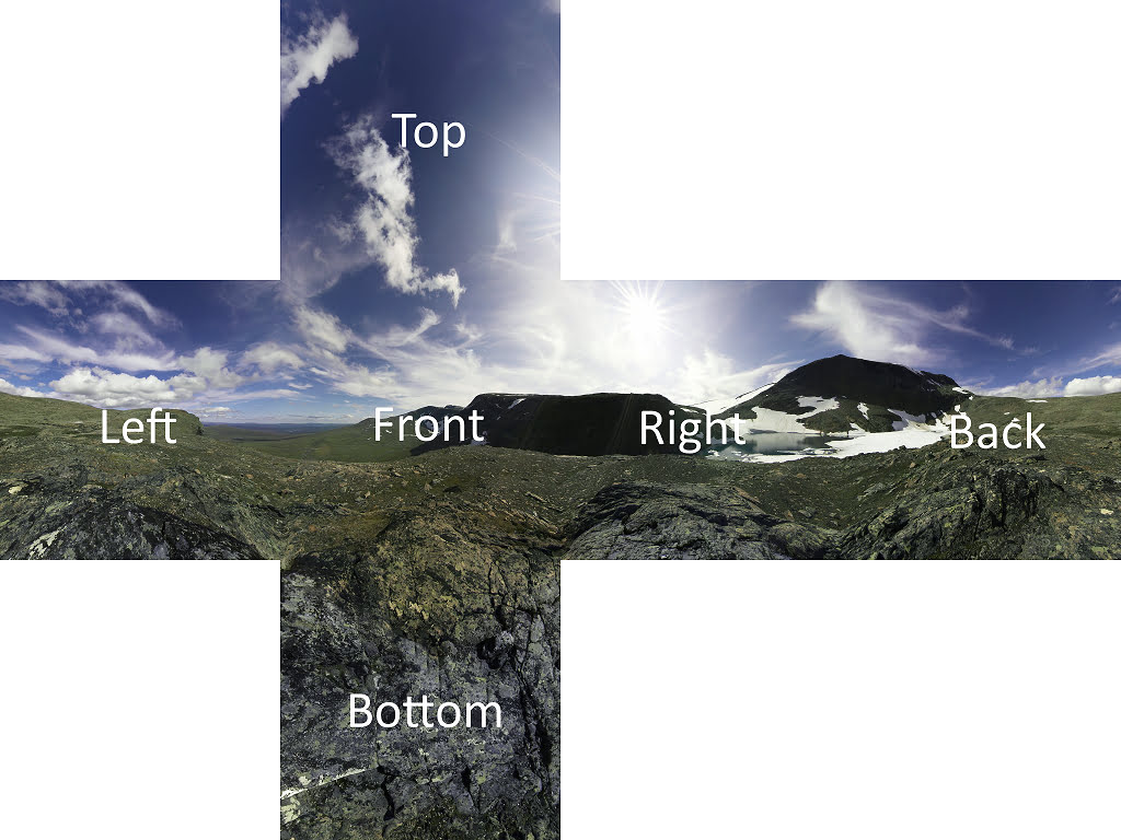
Specifies a single image that contains all 6 sides of a cube that encloses the scene (Figure 33).
The cubemap image must look similar to the following:
This cubemap image is the work of Emil Persson, aka Humus and is available under the Create Commons Attribution 3.0 Unported License: http://creativecommons.org/licenses/by/3.0/
Sometimes cubemap images are labelled as Min/Max XYZ faces. This can become confusing if the images are specified in a coordinate system where Y is up, as the Results applications treats the Z axis as up. To determine if the images are specified in an alternate coordinate system, find the bottom image. If it is labelled as Min Y, it is using a Y-is-up coordinate system. To enter these images, swap the Y and Z images when entering them into the Edit Skybox Dialog.
Once a skybox has been chosen, the following properties are available:
A screenshot is a still image of the scene. The Results application can create a single screenshot or multiple screenshots from different views and playback times.
To create a screenshot or series of screenshots, perform the following:
The following options are available for screenshots:
width x height.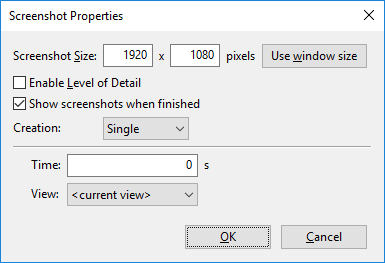
The Single creation method allows one screenshot to be created. The following options are available:
The Multiple creation method allows multiple screenshots to be created from several different playback times and views.
The following options are available:
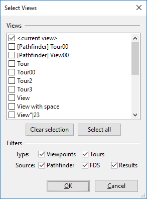
The Select Views dialog can be used to select which views the screenshots will be taken from. The list of views can be limited by unchecking the boxes next to the various filters at the bottom of the dialog.
When using the Multiple creation method, the screenshots are created in the following way: for each playback time between the start and end times using the time interval, a screenshot will be created for each selected view.
This means that there may be up to m*n screenshots taken, where m is the number of times between the start and end time, and n is the number of selected views.
The actual number of screenshots may be fewer than this, as screenshots will only be taken for a tour if the playback time is inside the time range of the tour.
The names of the screenshots follow this format:
name_time_viewname.ext
Where name is the name of the screenshot as chosen when the screenshot dialog was opened, time is the playback time for the screenshot as an offset in seconds from the start of the results, viewname is the name of the view from which the screenshot was taken, and ext is the image extension.
If <current view> is chosen as one of the views, _viewname is excluded from the file path.
Screenshots may also be created from a specification file. This method gives the most flexibility and allows the re-use of that specification between results visualizations, but it also requires the user to create the file.
To do so, create a file with the extension, .tsv, which stands for "tab-separated values".
This is a plain-text file, meaning that it can be created in a text editor, such as Notepad or Wordpad.
The format of the file is as follows:
time1 viewname1 viewname2
time2 viewname1 viewname3 viewname4
time3 viewname2
...
Each row specifies a different playback time, with the playback time in the first column. Each column after that specifies the name of a view.
If there are multiple views from different sources (e.g. Pathfinder or PyroSim) that have the same name, prepend the name with [Pathfinder] for views created in Pathfinder or [FDS] for views created in PyroSim and Pathfinder or Smokeview (do not include the quotation characters).
There must be a space after the closing square bracket.
Here’s a snippet from a file named screenshots_for_model1.tsv:
0.0 Top Front
30.0 \"Floor 0\" Left
120.0 Top
Selecting this file with a screenshot name of model1.png would create the following screenshots:
model1_000.000_Top.pngmodel1_000.000_Front.pngmodel1_030.000__Floor 0_.pngmodel1_030.000_Left.pngmodel1_120.000_Top.pngNotice that the quotation marks in Floor 0 turned into underscores (_).
The Results application does this to special characters that are not allowed in file paths.
Screenshots can also be created by running Results through the command-line without having to go to through the Results user-interface. This is useful, for instance, in automating the creation of screenshots for a report. This option supports all of the above ways of creating screenshots, including single screenshots, screenshots from multiple views at regular intervals, and screenshots from a tsv file.
In order to create screenshots this way, first open a command-prompt by clicking the Start menu, typing cmd, and pressing Enter.
To create a single screenshot, in the command-prompt enter:
"C:\Program Files\Pathfinder\PathfinderResults.exe" -screenshot -ssname "screenshots/ModelScreenshot.png" -sswidth 1280 -ssheight 720 -ssview "Entrance" -sstime 5.0 "C:\Pathfinder\test_model\test_model.pfrv"
This will create a single screenshot named C:\Pathfinder\test_model\screenshots\ModelScreenshot.png from the view, Entrance, at t=5.0 s. The screenshot will have the size, 1280x720.
To create multiple screenshots as described in Multiple, in the command-prompt enter:
"C:\Program Files\Pathfinder\PathfinderResults.exe" -screenshot -ssname "screenshots/ModelScreenshot.png" -sswidth 1280 -ssheight 720 -ssviews "Entrance,[Pathfinder] View00" -sstbegin 10.0 -sstend 120.0 -ssdt 5.0 "C:\Pathfinder\test_model\test_model.pfrv"
This will create several screenshots from the views, Entrance and [Pathfinder] View00. In this case, the screenshots will be located in C:\Pathfinder\test_model\screenshots\, have base name, ModelScreenshot, and size, 1280x720. The screenshots will start at t=10 s, end at t=120 s, and be 5 s apart.
To create screenshots from a tsv file as described in From File, in the command-prompt enter:
"C:\Program Files\Pathfinder\PathfinderResults.exe" -screenshot -ssname "screenshots/ModelScreenshot.png" -sswidth 1280 -ssheight 720 -sstsv "screenshots/testtsvfile.tsv" "C:\Pathfinder\test_model\test_model.pfrv"
This will create screenshots from the visualization file, test_model.pfrv, by using the tsv file, C:\Pathfinder\test_model\screenshots\testtsvfile.tsv. In this case, the screenshots will be located in C:\Pathfinder\test_model\screenshots\, have base name, ModelScreenshot, and size, 1280x720.
The following is the full list of screenshot commands that can be used:
-ssname argument is omitted, the screenshots will be located in the same directory as the visualization file and the names will be based on the visualization file name. If the name contains spaces, surround x in quotes, for example, -ssname "My Screenshot.png".1920] Specifies the width of the screenshot(s). If omitted, 1920 is used instead.1080] Specifies the height of the screenshot(s). If omitted, 1080 is used instead.<current view>] Specifies the name of the view from which to take a screenshot when not using a tsv file. If omitted, the active view saved in the visualization file is used.-ssviews "View00,My View,View 3".-ssview, -ssviews, -sstime, -sstbegin, -sstend, -ssdt.When creating a screenshot, the chosen size is often different than the current 3d view size in Results. For this reason, the screenshot might not exactly match what is seen in the 3d view. This can be fixed by matching the 3d view size with the desired sceenshot size. In order to do so, on the View menu, click Set 3D Window Size, which will open the Edit 3D Window Size dialog as shown in Figure 36. In this dialog, set the Width and Height to the same size that will be used for the screenshot.
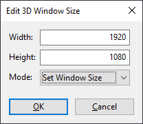
Click OK in the Edit 3D Window Size dialog to change the window size.
Movies can be created from the Results application for playback on machines that do not have the Results application or for presentation purposes. Movies can be created in two different ways. One way is to create a high-quality movie that is rendered offline. The other is to create a lower-quality movie in real-time that allows the user to interact with the scene while the movie is recording.
High quality movies are useful for presentation purposes, and play back smoothly at any resolution and with any high-quality settings turned on, regardless of the complexity of the scene. The disadvantage to this type of movie is that the camera must either remain static or its movements must be pre-planned using camera tours. In addition, the user cannot interact with the scene while the movie is being created (such as changing the selected occupant, turning on and off paths, etc.).
To create a high-quality movie:
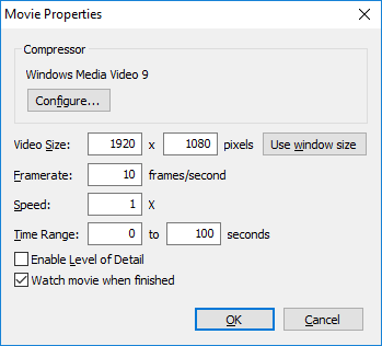
A dialog will show some movie making options as in Figure 37.
The options are as follows:
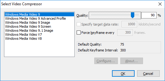
Shows which video codec is currently selected and allows the codec to be chosen and configured. If Configure is pressed, another dialog will show as in Figure 38. This dialog will show a list of the codecs currently installed on the computer. Some codecs allow certain properties, such as the Quality, Data Rate, and Keyframe interval to be specified. These properties control the resulting movie’s quality, file size, and seeking performance (how well a movie can be skipped around in the video player), respectively. Some codecs do not expose these properties through this dialog, however. To configure these codecs, you must press the additional Configure button if it is enabled.
 |  |
Movies can also be created in real-time. This means that it will record while the user is interacting with the results and it will record everything the user sees except for the cursor. The disadvantage of this type of movie is that it will play back only as smooth and of the same quality as that which the user who created the movie saw. So if the scene is very complex and the movie creator’s computer cannot view the results smoothly, the resulting movie’s play back will suffer as well.
To create a movie of this type, press the record button ![]() .
A file chooser dialog will prompt for the file name of the movie.
For real-time movies the only allowable type is WMV.
Once the file name is chosen, the codec configuration dialog will be shown as in Figure 38.
When OK is pressed on this dialog, the movie will begin recording.
At this point, anything the user sees in the 3D View will be recorded in the movie.
Now the user can change the camera angle, start and stop playback, select occupants, change view settings, etc. and the movie will capture everything.
At any time, the movie can be paused or stopped.
Pausing the movie will stop the recording but leave the movie file open so that recording can be resumed to the same file.
This allows the user to perform some action that they do not want to be recorded.
To pause movie recording, press the pause movie button
.
A file chooser dialog will prompt for the file name of the movie.
For real-time movies the only allowable type is WMV.
Once the file name is chosen, the codec configuration dialog will be shown as in Figure 38.
When OK is pressed on this dialog, the movie will begin recording.
At this point, anything the user sees in the 3D View will be recorded in the movie.
Now the user can change the camera angle, start and stop playback, select occupants, change view settings, etc. and the movie will capture everything.
At any time, the movie can be paused or stopped.
Pausing the movie will stop the recording but leave the movie file open so that recording can be resumed to the same file.
This allows the user to perform some action that they do not want to be recorded.
To pause movie recording, press the pause movie button ![]() .
To resume recording, press the resume movie button
.
To resume recording, press the resume movie button ![]() .
Stopping the movie will end recording and disallow any further recording to the file.
To stop recording, press the stop movie button
.
Stopping the movie will end recording and disallow any further recording to the file.
To stop recording, press the stop movie button ![]() .
.
In order to correctly preview what will be seen in the resulting movies, the 3D window size should match the size that will be used for the movie. This process is the same as it is for previewing screenshots. See Previewing Screenshots for more information.
Results can optionally be viewed in virtual reality using a VR headset, such as the Oculus Rift, HTC Vive, or other Steam VR-compatible headset. VR mode provides an immersive view of the model with a better sense of depth, object placement, and object sizes.
When VR Mode is activated, the roam tool is automatically selected and is the only tool that can be used to navigate the model. The viewing camera tracks the movements and orientation of the headset as the user looks around the model.
It is also possible to move through the model using the conventional mouse and keyboard controls for the roam tool, but it is not recommended, as moving the camera in this way can lead to nausea in some users.
VR Mode can also be started while a tour is active. It is recommended that the tour consists only of stationary viewpoints to avoid nauseating the user. When done this way, viewpoints will fade in and out to avoid sudden transitions for the user. If the tour does include camera movements, it will act as if the user is sitting in a car that is moving on rails, allowing the user to continue looking around the model as the tour progresses.
The following headsets have been verified to work with the Results:
It should, however, work with several other headsets, including all that are compatible with Steam VR and Oculus PC platforms, including the Oculus Rift S, HTC Vive Pro, Valve Index, Samsung Odyssey, etc.
The computer also needs a high-performance video card and processor. Typical VR computers tend to have the following specifications:
Many vendors supply VR-Ready machines as well.
To use VR Mode in the Results, perform the following steps:
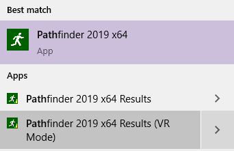
While not wearing the headset, run Results using the Pathfinder VR Mode shortcut from the Start menu Figure 39.
Verify that there is a VR button in the main toolbar as shown in Figure 40. If it is greyed out, see VR Troubleshooting.
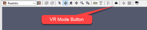
Click the VR button ![]() , click play on the timeline, and put on the VR headset.
Depending on the headset, it may take up to a minute for the Results to appear in the headset.
Once it does start displaying, the headset should show the viewpoint inside the model with the data being displayed.
You can now look and move around in the model with the view updating continuously as your head is moved.
, click play on the timeline, and put on the VR headset.
Depending on the headset, it may take up to a minute for the Results to appear in the headset.
Once it does start displaying, the headset should show the viewpoint inside the model with the data being displayed.
You can now look and move around in the model with the view updating continuously as your head is moved.
The Results window should show the user’s viewpoint from each eye as shown here:

There are some limitations to using VR mode:
Views provide the capability to store and retrieve various view state in the Results, to create animated tours of the model, and to clip the model and results using section boxes.
There may only be one active view at a time. There is always a Default view, which contains no saved state and is the active view by default. Whenever a view is activated, the stored view state will be restored. View state may optionally include any of the following:
A view may have a viewpoint or tour, but not both. A section box can be used in combination with either, however.
To activate one of the views, either double-click the desired view in the navigation view or right-click it and select Set Active. This will make the view active and restore the view state associated with that view.
If there is a tour or section box, the tour/section box becomes active and remains active as long as the view is active. If there is a viewpoint instead of a tour, the camera shows the viewpoint, but the navigation tools can still be used to modify the camera. Modifying the camera does not modify the saved viewpoint, however.
To deactivate the view, either double-click the active view or right-click it and select Set Inactive. This activates the Default view. Alternatively, another view can be made active, which will automatically deactivate the currently active view and make the new one active.
If any views or tours were created in PyroSim, Pathfinder, or Smokeview, they will appear in the navigation view, with a label indicating their origin, such as [Pathfinder] or [FDS]. While these views cannot be edited, they can be duplicated, and the duplicates can be edited. For more information, see Duplicating Views.
At any time, the state of the active camera can be saved to a view, including its position, orientation, and zoom. A viewpoint can be recalled later to view the scene from that perspective.
A viewpoint can be created in one of the following ways:
This will add a new view to the model, saving the current camera viewpoint, section box, navigation tool, and camera type (Perspective versus Orthographic) into the new view. The new view will become the active view.
To delete a view, select it in the navigation view and press Delete on the keyboard. If the deleted view was active, the default view becomes active instead.
To recall a viewpoint, perform any of the following:
Recalling a viewpoint will switch the scene camera to either the perspective camera or orthographic camera and will initialized it with the state of the saved viewpoint. In addition, the saved navigation tool will also become active.
If the orientation of a viewpoint needs to be changed, perform the following:
This will save both the current camera orientation and navigation tool into the view.
The Results application provides the capability to create and view camera tours, which can be played back or recorded to video.
Tours are useful in the following scenarios:
Conceptually, camera tours consist of a number of viewpoints at different playback times, referred to as keyframes. When a tour is played back, the scene camera smoothly interpolates between viewpoints at the keyframes. Tours may repeat and can start at any time.
When a tour is active, the results playback time range is set to the time range of the tour (Results Timelines).
Tour creation and editing is performed through the Tour Editor Dialog, as shown in Figure 42. The tour editor dialog allows various tour properties to be modified and allows keyframes to be added, removed, and modified.
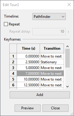
While the tour editor dialog (Figure 42) is open, the scene camera will stop tracking with the tour. This is to allow positioning of the camera in order to add or edit keyframe positions. To preview changes made to the tour, click the Preview button at the bottom of the tour editor dialog. This will lock the scene camera back to the tour and begin playback at the current time. If the current time is outside the tour time or at the end of it, the playback time is changed to the beginning time of the tour. To end the preview, click End Preview. The scene camera will once again unlock, allowing changes to the keyframes.
While the tour editor dialog is open, clicking a keyframe in the table will also set the playback time of the results to that keyframe time and show the viewpoint of that keyframe in the 3D view. Similarly, changing the scene playback time using the time slider will automatically select the most recent keyframe in the table.
While the tour editor dialog is open, another view can be double-clicked in the navigation view to show the viewpoint of that view.
Tours have the following properties:
Keyframes have these properties:
Specifies how the scene camera will transition to the next keyframe. If this is the last keyframe and Repeat is checked, the next keyframe is the first keyframe.
The transition value can be one of the following:
To create a tour, perform the following:
In the 3D view, right-click empty space and select New tour.
There will be times when changes need to be made to a tour, such as the start time, camera position during a transition, adding a repeated section of the tour, etc. Tours can be edited in several ways.
To begin editing the tour, open the tour editor dialog in one of the following ways:
With the tour editor dialog open, several changes can be made, including the following:
Sometimes a keyframe doesn’t have quite the right orientation or camera position. This can be changed by doing the following:
Perhaps all the keyframes look correct, but there is a point in the tour when the camera does not look quite right. This can be fixed by doing the following:
A portion of the tour can be removed by deleting keyframes. To do so, select the keyframes and either press Delete on the keyboard or right-click the frames and select Remove.
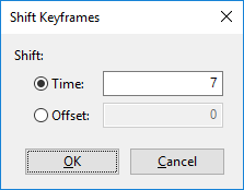
There might be scenarios where all or part of a tour needs to be moved to a different time. If the time of only one keyframe needs to be corrected, edit the time value directly in the Keyframes table. If all or a portion of the tour needs to be shifted:
The selected keyframe times will be shifted by the specified amount.
If you want to duplicate some or all of the tour so that the section will play again at another time within the same tour, perform the following:
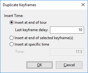
After creating a tour, it may be decided that the camera should remain stationary at a particular viewpoint for some length of time before moving on to the next keyframe. This can be done by duplicating the keyframe that should be held and selecting Insert at end of selected keyframe as described above.
The new keyframe will have the same viewpoint as the previous keyframe, which keeps the camera stationary before moving on to the next keyframe. While not completely necessary, it may also be desirable to set the old keyframe transition to Stationary to make it obvious in the keyframes table which keyframe is being held.
A section box is a convex region defined by up to six planes and is used to limit the scope of visible geometry and results data. All data outside the box are clipped from view. An example of the clipping is shown in Figure 46.
 |  |
NOTE: When viewing a section box with the floors of the model spread out, each floor is clipped by the intersection of the section box and the Z clipping planes of the floor. See Viewing Multi-floor Problems for more information on floors.
The active view’s section box can be disabled by going to the View menu and de-selecting Views and Tours→Enable Section Boxes.
A section box can be created in several ways:
After a section box is added, the Section Box Dialog appears as shown in Figure 47.
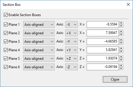
While the section box dialog is open, the section box is displayed as a dashed outline of the region with translucent faces. The individual planes of the section box can be added and removed by checking and unchecking the box next to each plane.
A section box can be edited in several ways:
A section box can be removed from a view in any of the following ways:
With the exception of the default view, any view can be duplicated, including those from Pathfinder, PyroSim, or Smokeview. To duplicate a view or several views:
This will create a copy of each view. All duplicated views can be modified and deleted.
Views made in Pathfinder, PyroSim, Smokeview, and Results versions 2019.1.0515 and prior are stored in several different files including the following:
modelname_views.json - Views file created in Pathfinder.
This is saved in a JSON file format.modelname.views - Views file created by PyroSim.
This is also saved in a JSON file format.modelname.ini - File created by PyroSim or Smokview that contains viewpoints and tours created for use in Smokeview.modelname_resultsviews.json - Views file created by the Results application in versions 2019.1.0515 and prior for storing views created in the results, including those duplicated from PyroSim, Pathfinder, or Smokeview views.
This is also stored in a JSON file format.Where modelname is the name of the originating Pathfinder, PyroSim, or FDS file.
Views can be imported into the results, for instance, from another results data set.
To do so:
The views are imported as editable results views into the current results visualization.
Results provides a special view mode to have the camera follow an occupant as they travel through the simulation.
To activate this mode, select the desired occupant, and then either click the Follow Occupant button ![]() in the main toolbar or right-click the occupant and select Follow Occupant. The camera will remain behind the occupant as results are played back. Activating this view mode will deactivate other views and tours. To stop following the occupant, click the Stop Following Occupant button
in the main toolbar or right-click the occupant and select Follow Occupant. The camera will remain behind the occupant as results are played back. Activating this view mode will deactivate other views and tours. To stop following the occupant, click the Stop Following Occupant button ![]() or right-click anywhere in the 3D view or navigation view and select Stop Following Occupant.
or right-click anywhere in the 3D view or navigation view and select Stop Following Occupant.
The Results application provides several different ways to annotate results, including the ability to add dimensions and custom labels.
Annotations are added by drawing them directly into the model using one of the provided tools, detailed below. This can be accomplished in either the Perspective View or Orthographic View, though in some cases it may be easier to use one over the other.
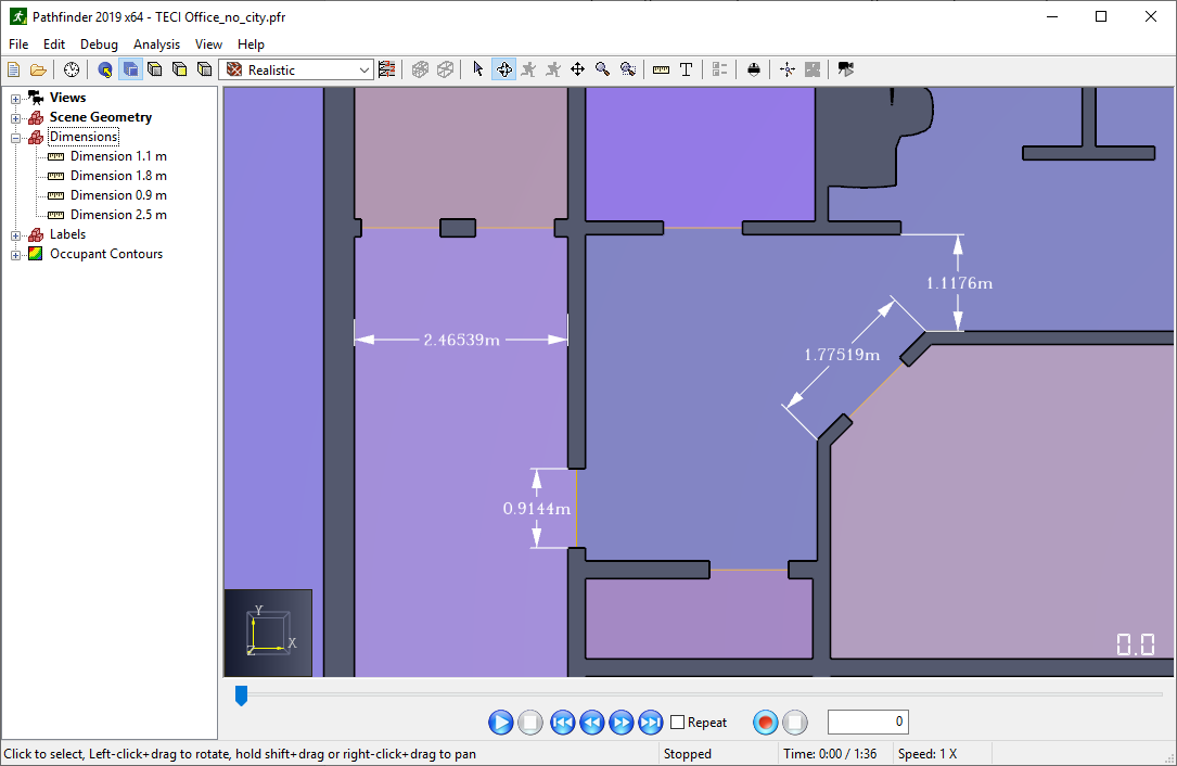
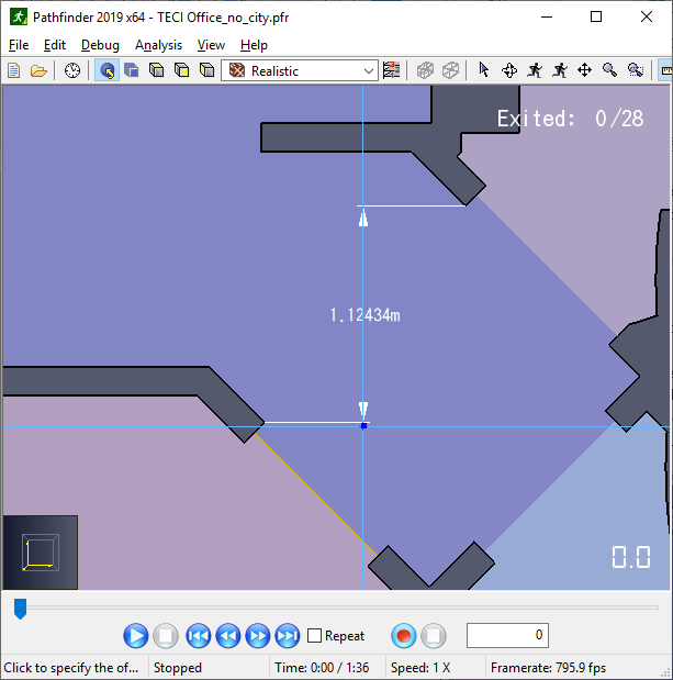
Dimensions may be added to a results visualization to annotate the length of features in the model or distances as shown in Figure 48. Dimensions may be shown or hidden by going to the View menu and selecting or deselecting Show Dimensions. Go to File › Preferences › Dimensions and Precision, to adjust the total precision of the dimension.
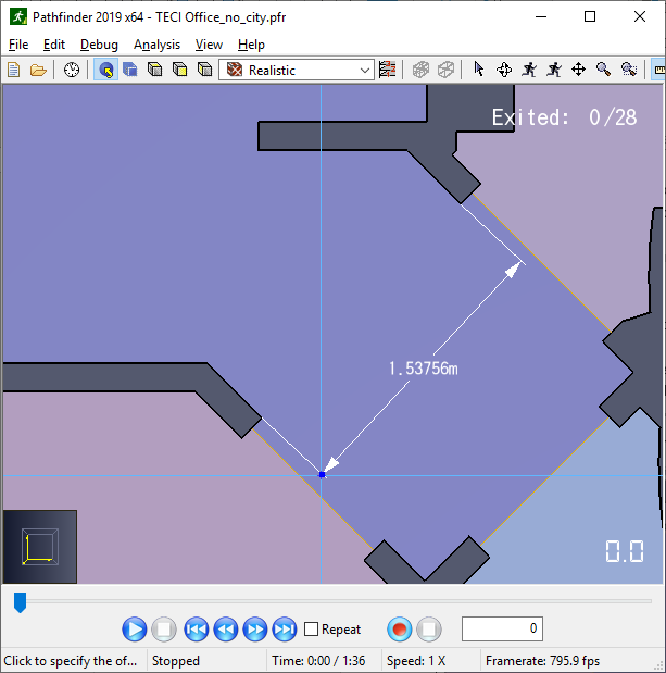
To draw a dimension, perform the following steps:
Click the Dimension Tool ![]() button in the toolbar above the 3D view to start drawing.
button in the toolbar above the 3D view to start drawing.
When pinned, the dimension tool will stay active until Esc is pressed on the keyboard, allowing multiple dimensions to be drawn, one after the other. If the tool is unpinned, the most recently used navigation tool will become active after a dimension is drawn.
The resulting dimension is parallel to the feature and matches its length as shown in Figure 50. To dimension in this manner, move the cursor along an imaginary line extending from the second dimension point and perpendicular to the dimensioned feature.
Dimensions may be selected and deleted from either the 3D view or the Navigation View under the Dimensions group.
 |  |
 |  |
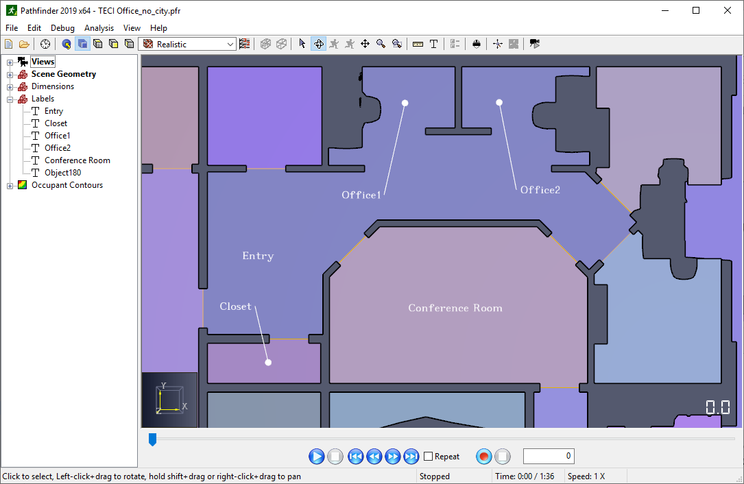
Another way to annotate results is to add custom labels as shown in Figure 53. Custom labels can be used to add any text to the model and can be added with or without a leader. Labels may be shown or hidden by going to the View menu and checking or unchecking Show Labels.
To create custom labels, perform the following steps:
As with dimensions, labels appear in the Navigation View under the Labels group and can be deleted or renamed if necessary.
The Results application provides support for viewing results from the Fire Dynamics Simulator (FDS) from NIST. It is the default results viewer for PyroSim, which is a graphical user interface for FDS. FDS results may optionally be shown along with Pathfinder results. When FDS results are loaded, the Navigation View will list all of the supported FDS output as shown in Figure 54.
The Results application supports the following FDS output:
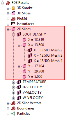
Each FDS output may be split into multiple objects depending on how many meshes the object resides in. Figure 55 show an example model where there are multiple meshes. In this example, there are five slices of SOOT DENSITY at different locations. The slice at X=13.319 only goes through one mesh, so there is only one entry in the Navigation View. The slices, X=13.5 and Y=17.104, however, go through multiple meshes, so they have multiple entries in the Navigation View.
The hierarchy in this view makes it easy to activate an entire slice as it goes through multiple meshes or only activate the slice in one or more meshes. It also demonstrates how individual results objects have been divided among multiple meshes.
When an FDS results file is loaded, none of the results are visible. They must be selectively activated to be shown. To do so, in the Navigation View either right-click the desired results object and select Show or double-click the object. To deactivate the object, right click it and select Hide or double-click it.
Results objects can be activated or deactivated at any level in the hierarchy.
For instance, in Figure 55, all SOOT DENSITY slices can be activated by double-clicking SOOT DENSITY in the navigation view.
In addition, all SOOT DENSITY slices at X=13.5 can be activated by double-clicking X = 13.5000.
Note that only one FDS quantity can be active at a time.
For instance, a TEMPERATURE slice may NOT be shown along with a SOOT DENSITY slice.
You can, however, mix different result types as long as they are the same quantity.
For instance, you can show a TEMPERATURE slice and a TEMPERATURE boundary.
The exception to this rule is that 3D Smoke and Particles colored with the Default color can be shown in combination with any quantity.
This is because these outputs have no associated quantity.
When an object is activated the Results application performs several actions:
SOOT DENSITY slice X = 13.5000 : Mesh 3 is activated, the Navigation View will appear as shown in Figure 56.
This makes it easy to see which items in a hierarchy are currently active even if a node is collapsed.tcframes. For instance, if particles are loaded from a file named carport.prt5, the caching file will be named carport.prt5.tcframes.tcframes file.
This occurs much faster than loading the first time.
In addition, the application checks to see if there are new frames in the object’s file, which can occur if the FDS simulation is still running.
If there are more frames, information is gathered for only the new frames and added to the cache file.SOOT DENSITY slice is already active and a TEMPERATURE slice is being activated, the SOOT DENSITY slice is deactivated.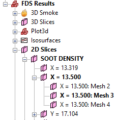
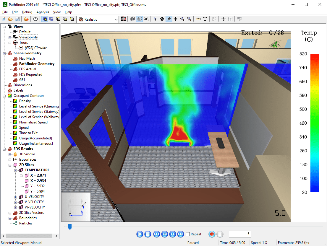
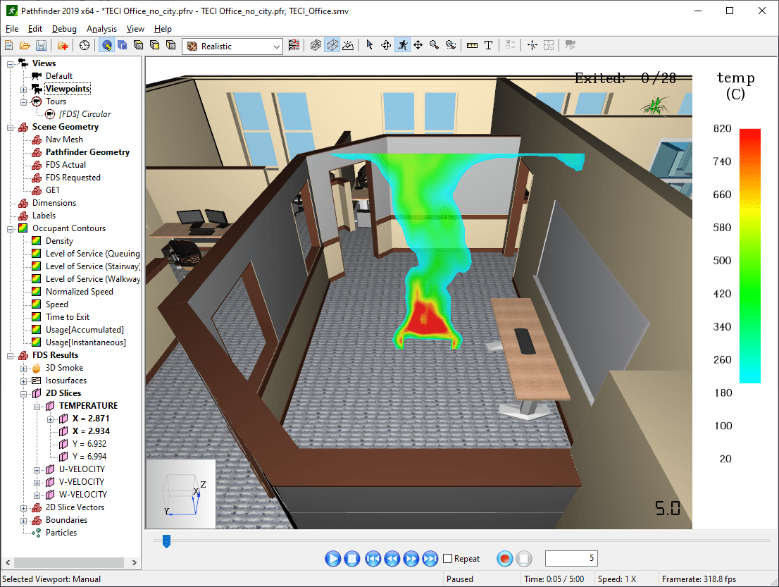
Nearly all FDS and Pathfinder results data are colored with a colormap (exceptions include 3D Smoke, Particles viewed with the Default coloring, and some occupant coloring options).
A colormap provides a way to map data values to a color that can be displayed on the screen.
When a colormap is in use, it will be shown as a colorbar on the right side of the 3D View as shown in Figure 57. If both FDS Results and Pathfinder occupant contours are displayed at the same time, there may be multiple colorbars displayed at once.
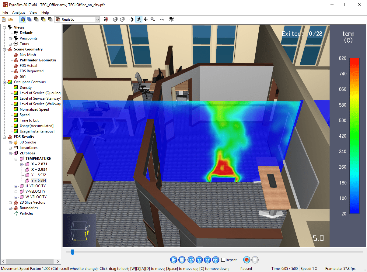
The colorbar shows the colormap as well as which data values are mapped to the colors.
At the top, it also shows an abbreviation of the quantity and the quantity’s unit in parentheses.
In Figure 57, the label "temp" corresponds with the quantity, TEMPERATURE, and the unit is C for degrees Celsius.
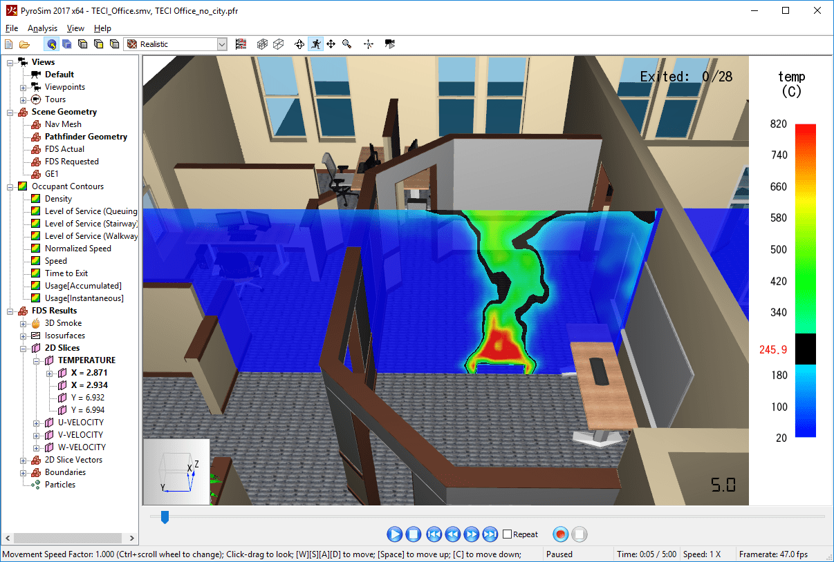
The colorbar can be left-clicked to add a highlight region. A highlight region changes all of the values of a limited range to a specific color to make it easier to see as shown in Figure 58. By default, a highlight region covers 5% of the data values surrounding the clicked location on the colorbar (2.5% above and 2.5% below). The size of the region can be changed by using the scroll wheel on the mouse. In addition, the highlight region can be removed by right-clicking the colorbar. The highlight region can also be moved by clicking and dragging the left mouse button on the colorbar.
More fine-grained control over the colorbar can be achieved by double-clicking the colorbar, which will bring up a dialog to edit the colorbar properties as described in Colorbar Properties.
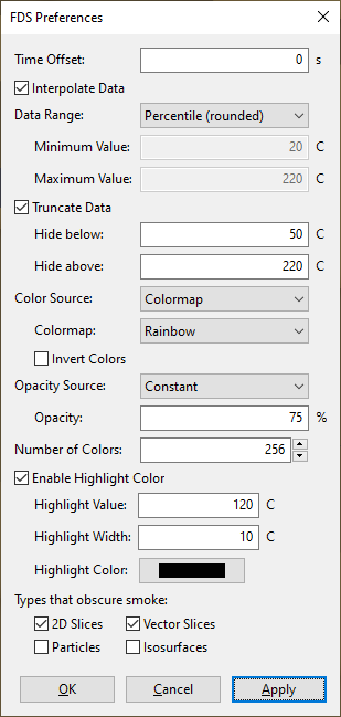
Colorbar properties are edited in either the FDS Preferences dialog as shown in Figure 59 or the Occupant Contour dialog as shown in Figure 100. Either dialog can be reached by double-clicking the colorbar.
x% of contour values from opaque to transparent so that the underlying geometry or navigation mesh may be seen. Values above the threshold are opaque. For example, if the data range is 0-10, and the Feather Threshold is 25%, values below 0 will be transparent, values in the range 0-2.5 will increase in opacity until they are opaque at 2.5, and all values above 2.5 will be opaque.x% of contour values from opaque to transparent so that the underlying geometry or navigation mesh may be seen. Values below the threshold are opaque.The opacity at the Minimum Value as specified in the Data Range. This can be any value and does NOT have to lie between 0 and 100%.
 |  |
There is a set of global properties for FDS results that controls how the results are presented, including the colorbar properties, time offsets, and interpolation. These settings are located in the FDS Preferences dialog. To open this dialog, either double-click the colorbar if results are already active or under the Analysis menu, select FDS Preferences. The FDS Preference dialog is shown in Figure 59.
In addition to the colorbar properties explained in Colorbar Properties, the following options are available in the FDS Preferences dialog:
Indicates that results should be linearly interpolated over time. This causes the animation of results to look smoother as they are played back.
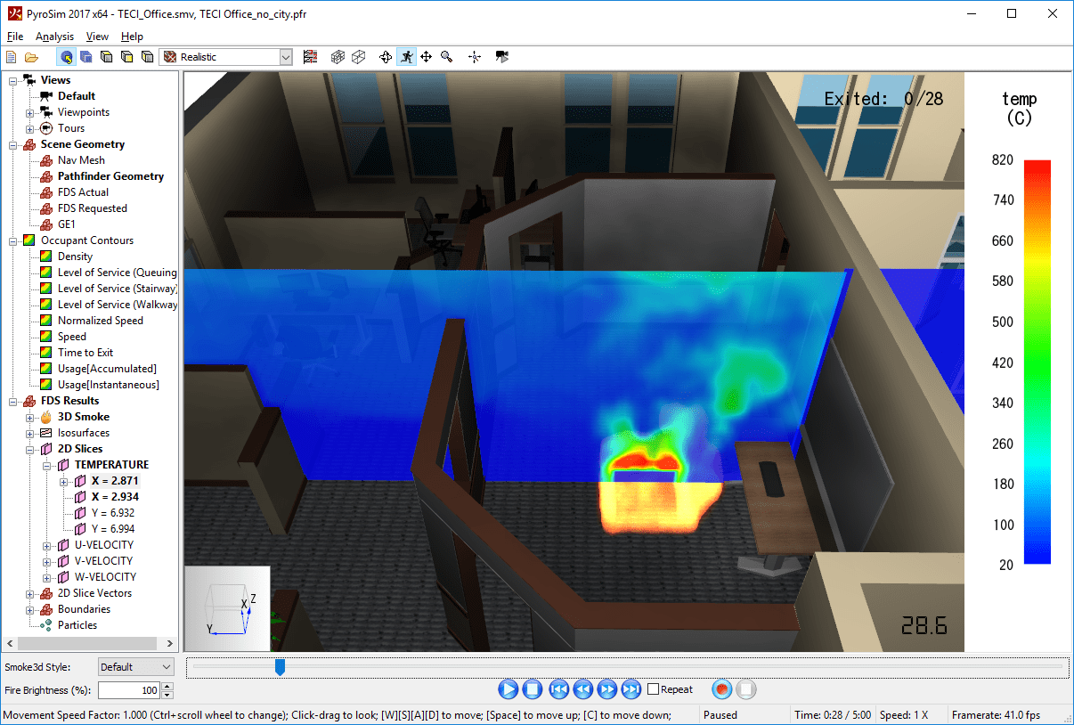 | 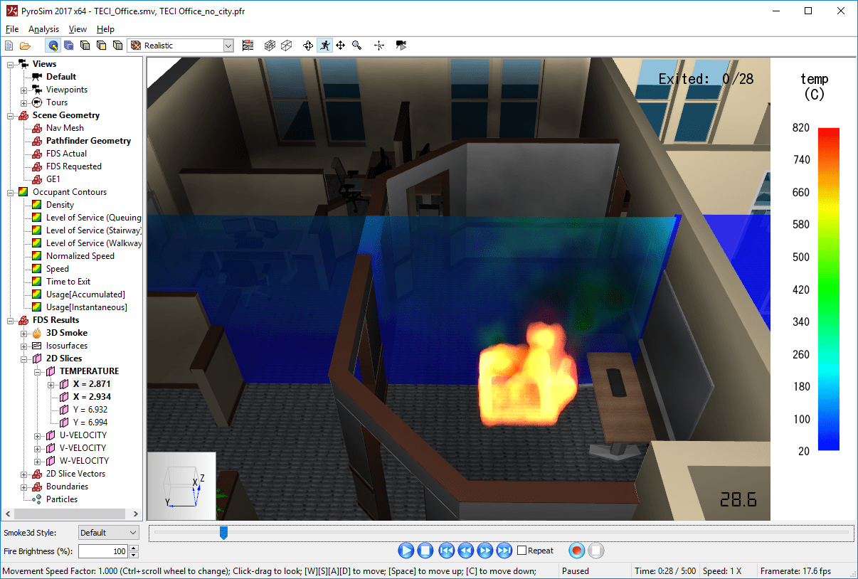 |
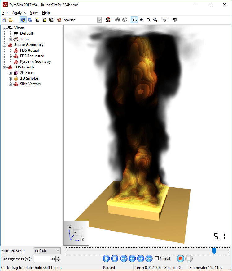
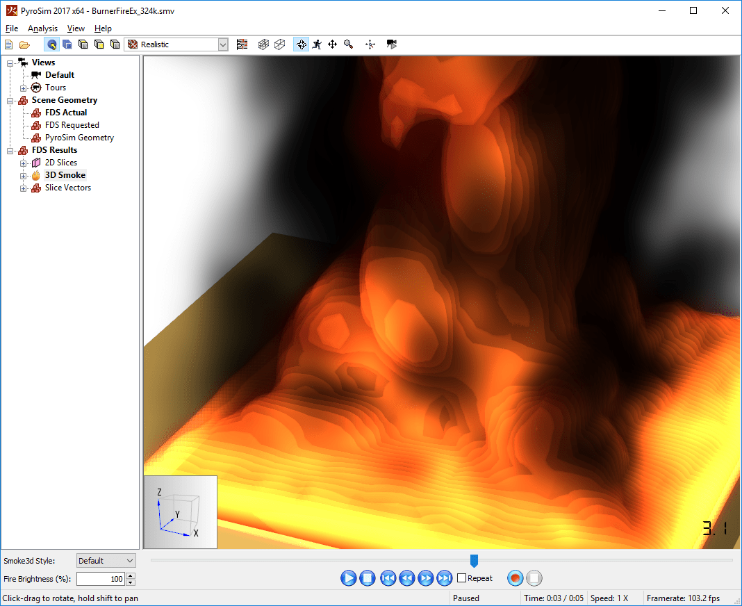
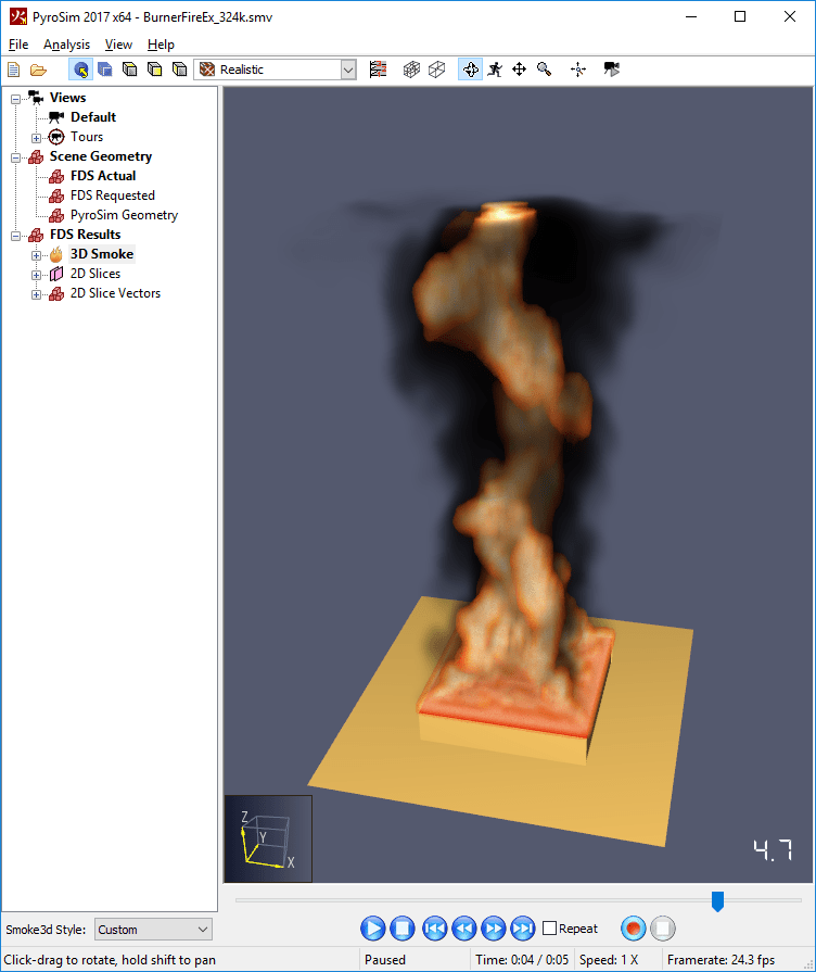
By default, all FDS simulations that contain fire will output two s3d files for each mesh. Together these files can be viewed in the Results application as smoke and fire as shown in Figure 64. When these files are present, the Results application will show a 3D Smoke group in the Navigation View. In the 3D Smoke group, SOOT MASS FRACTION represents the smoke information and HRRPUV (heat release rate per unit volume) represents the fire information.
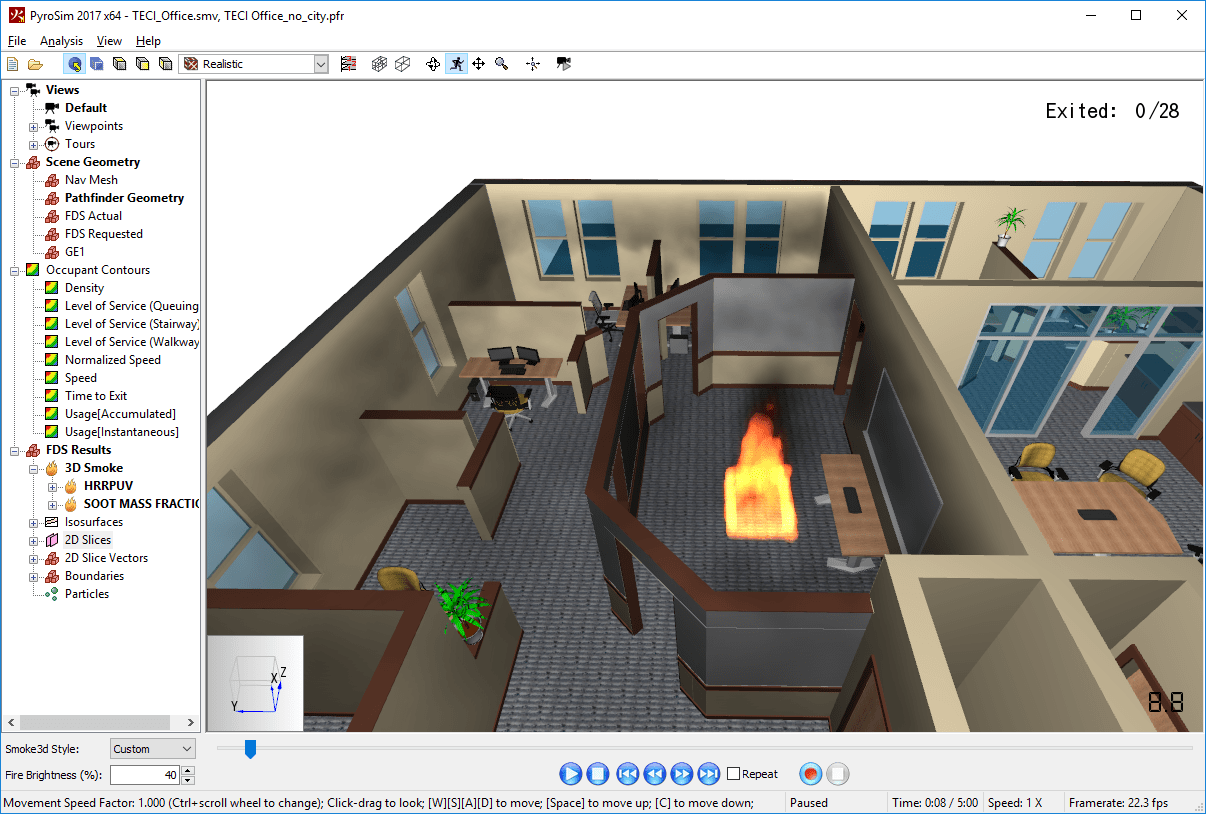
The smoke and fire visualization is merely an approximation of the actual smoke and fire.
The visualization has the following limitations:
There are a number of properties that affect the appearance of the smoke and fire. These properties can be edited by right-clicking the 3D Smoke group in the Navigation View and selecting Properties. This will show the Smoke3D Properties dialog in Figure 65.
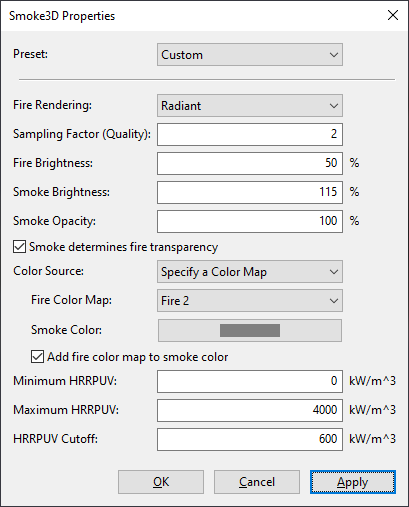
Approximates real fire, where the fire itself emits light and accumulates along the view ray toward the camera, while being absorbed by smoke between the viewer and the fire. Usually when using this option, Smoke determines fire transparency should also be checked.
If Fire Rendering is set to Radiant, this controls how bright the fire appears. This is similar to adjusting the exposure on a camera, except that it only affects the light from the fire. If the fire appears almost completely white, this may be because it is either a very large fire or has little smoke. In this case, lower the brightness. If the fire can barely be seen, it may be because of very thick smoke. In this case, increase the brightness.
Controls how opaque the smoke appears.
The color of the smoke. The final smoke color may be adjusted by also adding in color from the fire color map. See Add fire color map to smoke color below.
Controls how cells are determined to be smoke or fire cells. If the HRRPUV value is less than HRRPUV Cutoff, the cell is treated as a smoke cell and only absorbs and reflects light (reflection color is the smoke color). All other cells are treated as fire cells. If Fire Rendering is set to Radiant, these cells will absorb light and emit light as determined by the colormap.
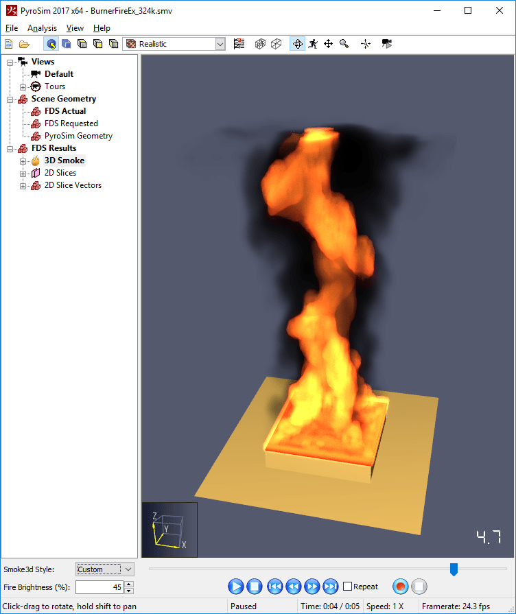 | 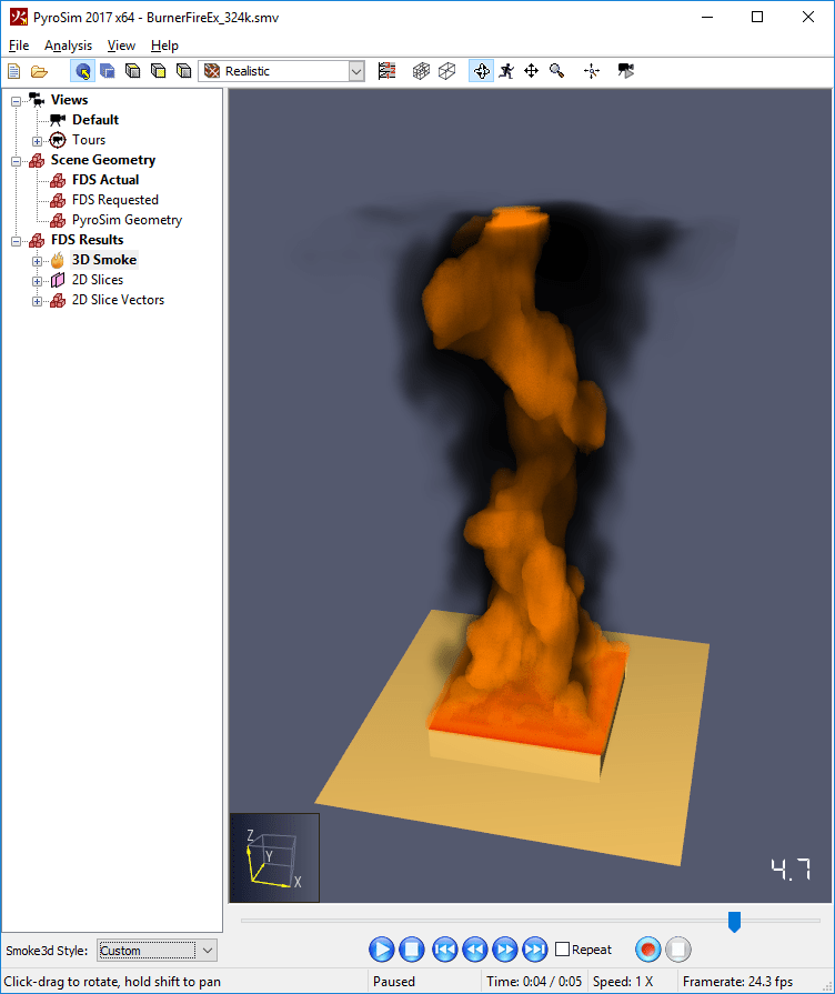 |  |
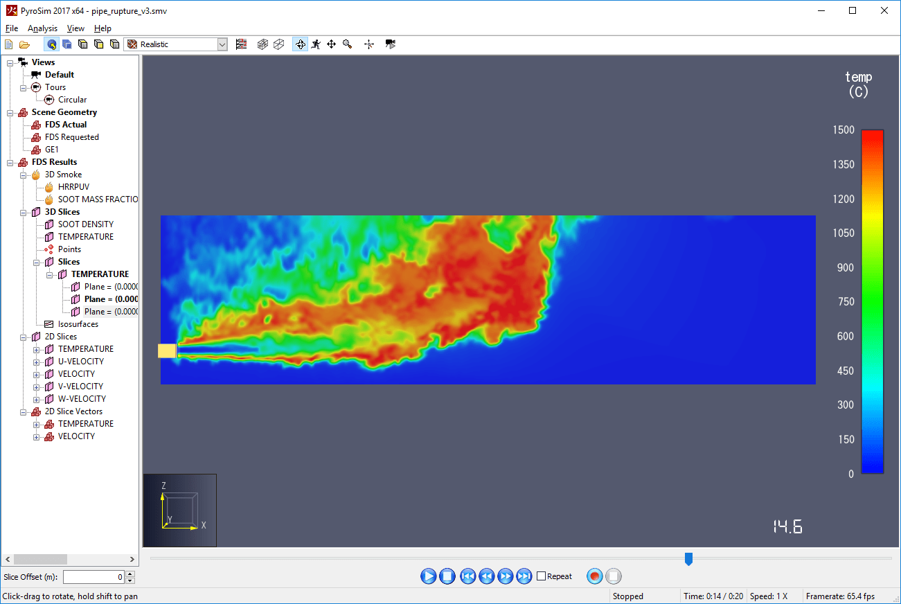
In FDS, a 3D slice represents an animated volumetric region that contains data at every intersecting cell for a single gas-phase quantity such as TEMPERATURE or SOOT DENSITY. There can be any number of 3D slices of the gas-phase quantities.
When an FDS simulation contains 3D slices, they will appear under the 3D Slices group in the Navigation View. The hierarchy appears in the Navigation View as FDS Results→3D Slices→Quantity→Mesh.
For more information on the visualization capabilities of 3D slices, refer to Data3D.
FDS has the capability of creating Plot3D files. Like 3D slices, a Plot3D file contains 3D data sets. There are a few key differences between the file format for Plot3D and 3D slices:
Despite the differences, the Results application hides these details from the user and presents Plot3D output exactly like 3D slices, in that each quantity is represented as a separate object in the Navigation View. In addition, the Results application will treat all of the Plot3D files of a given quantity as if they were one animated file.
When an FDS simulation contains Plot3D data, they will appear under the in the Navigation View with this hierarchy: FDS Results→Plot3D→Quantity→Mesh.
For more information on the visualization capabilities of Plot3D, refer to Data3D below.
Both Plot3D and 3D slice files contain 3D datasets (Data3D) of gas-phase quantities. Though they require fairly significant storage space, Data3D are perhaps the most flexible output formats from FDS and can be visualized in several ways.
They can be viewed directly using volumetric rendering, and arbitrary isosurfaces, slices, and points be created from them in the Results application without being required to re-run the FDS simulation.
Volumetric rendering of a Data3D object enables viewing it as a 3D form as if it was a cloud of colored gas as shown in Figure 69.
In order to understand the shape and depth of the volume, portions of the dataset must be made translucent.
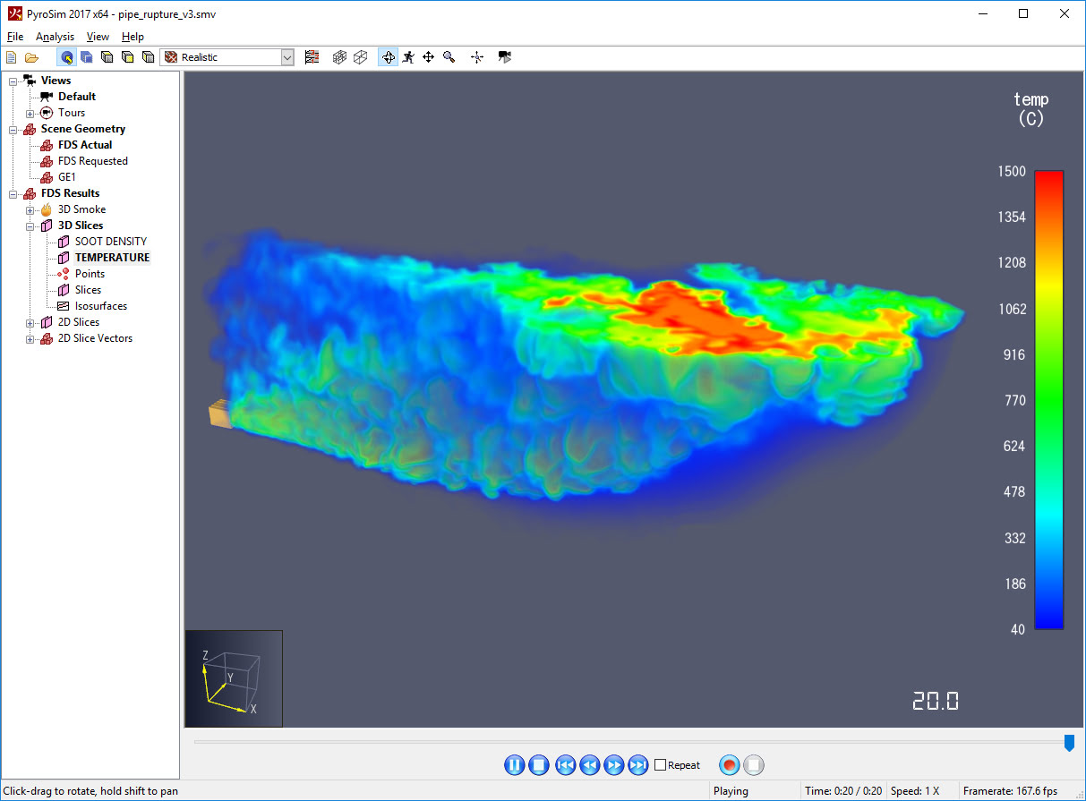
By default, the minimum value in the data range (Global FDS Properties) has an opacity of 0% making the lower values completely transparent. The maximum value in the data range has an opacity of 75%. The range of opacity values can be changed by either choosing the constant opacity value or by choosing a Gradiant Opacity Source in the FDS Preferences dialog and setting the desired opacity mapping.
Volumetric renderings are created similarly to fire and smoke. To change their quality, in the Navigation View expand either 3D Slices or Plot3D, right-click one of the quantities, and select Properties. This will open the Data3D Properties dialog as shown in Figure 70.
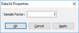
When using hardware shaders, the Sample Factor controls the number of samples taken from the data set for each view ray. When using the compatibility renderer, the Sample Factor controls the number of slices through the 3d texture. Increasing this value will generally increase the quality of the volumetric rendering at the expense of rendering speed.
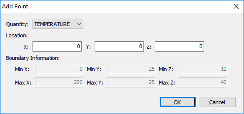
From Data3D objects, any number of points can be created that are colored according to the colorbar and Data3D values as shown in Figure 71. Data3D points can also be used to export time-series data and show plot from the Data3D object as explained in Exporting Data and Time History Plots.
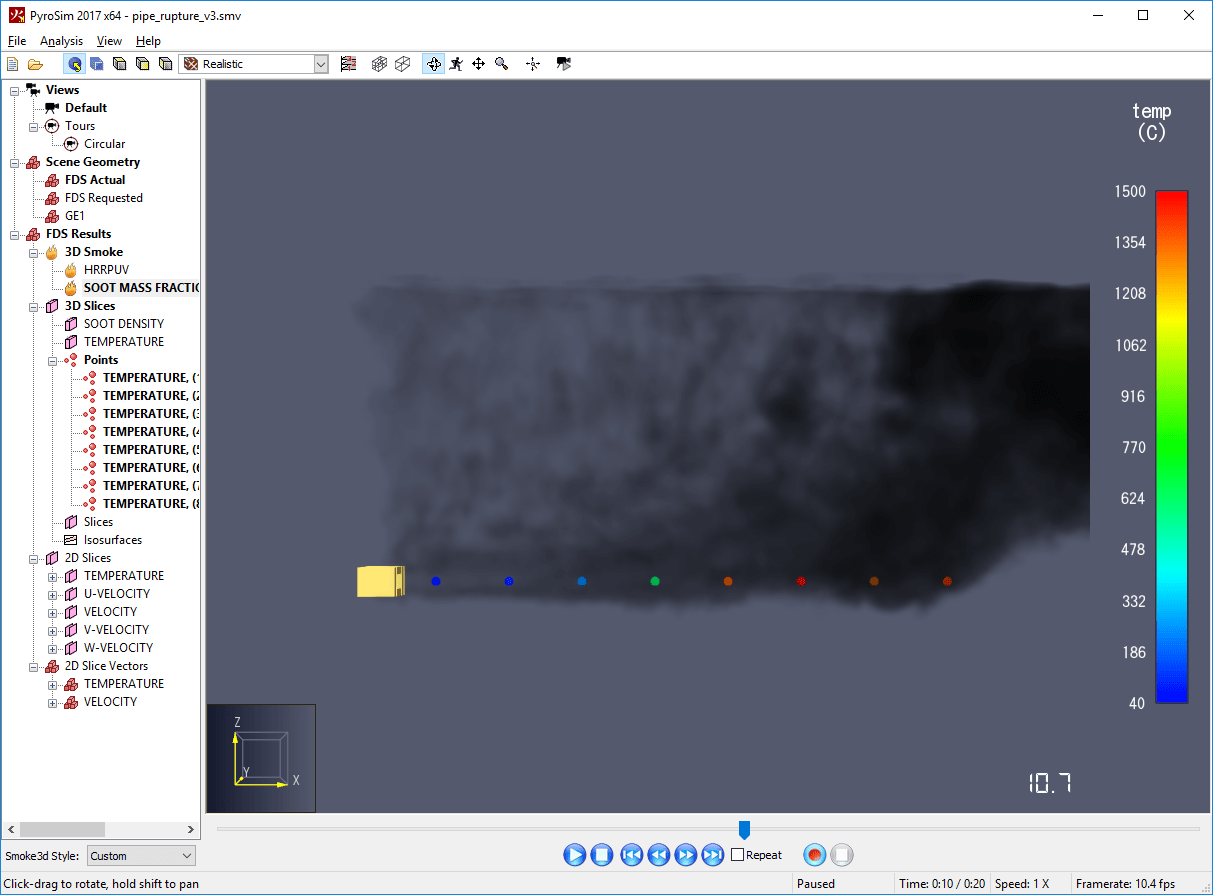
To create a Data3D point:
Choose the desired quantity and location of the point and click OK. The point will be added under the Points group.
To delete a Data3D point, select it in the Navigation View and press the DELETE key.
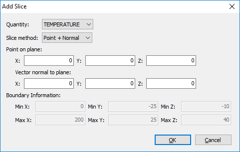
Arbitrary 2D slices can also be created from Data3D objects without rerunning the simulation. These slices do not have the same restrictions as regular FDS slices in that they do not have to be axis-aligned. Instead, they can be in any plane. Figure 73 shows a 2D slice created from a 3D slice.
To add a Data3D slice:
When Data3D slices are active, they can be quickly moved along their normal in the Quick Settings.
To delete a Data3D slice, select it in the Navigation View and press the DELETE key.
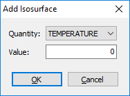
Arbitrary 3D isosurfaces can also be created from Data3D objects without rerunning the simulation. An isosurface shows the contour of a gas-phase quantity at a specific value. Some isosurfaces created from a 3D slice are shown in Figure 75.
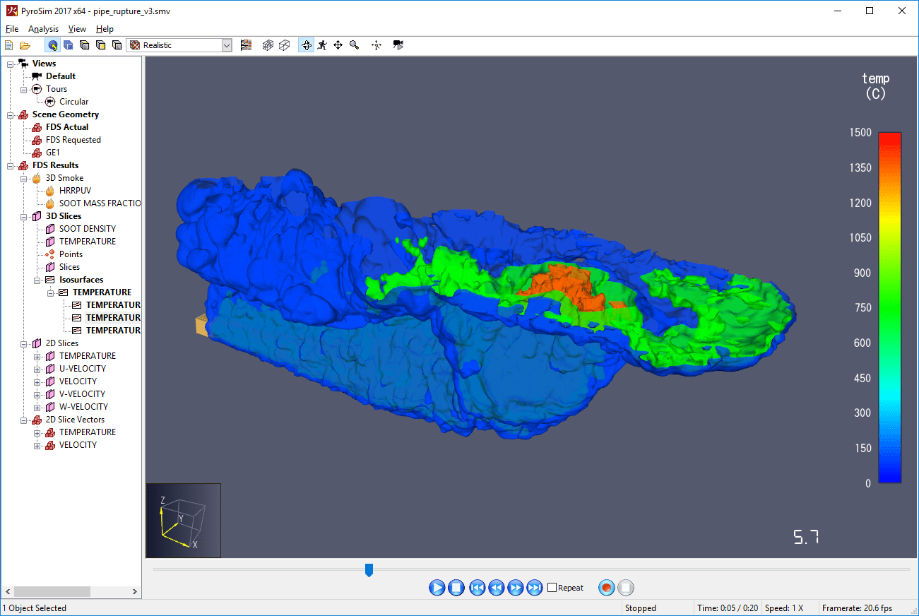
To add a Data3D isosurface:
If only one Data3D isosurfaces is active, its value can be quickly changed in the Quick Settings.
To delete a Data3D isosurface, select it in the Navigation View and press the DELETE key.
FDS supports the generation of animated 3D isosurfaces. An isosurface shows the contour of a gas-phase quantity at a specific value, as shown in Figure 77.
Unlike Data3D isosurfaces, FDS isosurfaces cannot be added or changed in the Results application. Instead, they must be specified in the FDS input file or in PyroSim.
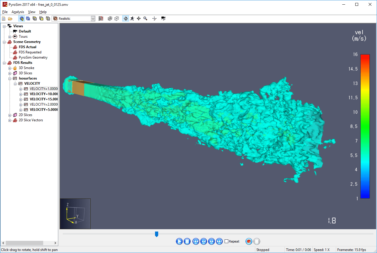
When an FDS simulation contains isosurfaces, they will appear under the Isosurface group in the Navigation View. The hierarchy appears in the Navigation View as FDS Results→Isosurfaces →Quantity→Value→Mesh.
FDS also supports the generation of animated 2D slices. A 2D slice shows the values of a gas-phase quantity in a single plane as shown in Figure 78.
Unlike Data3D slices, FDS 2D slices cannot be added or changed in the Results application. Instead, they must be specified in the FDS input file or in PyroSim.
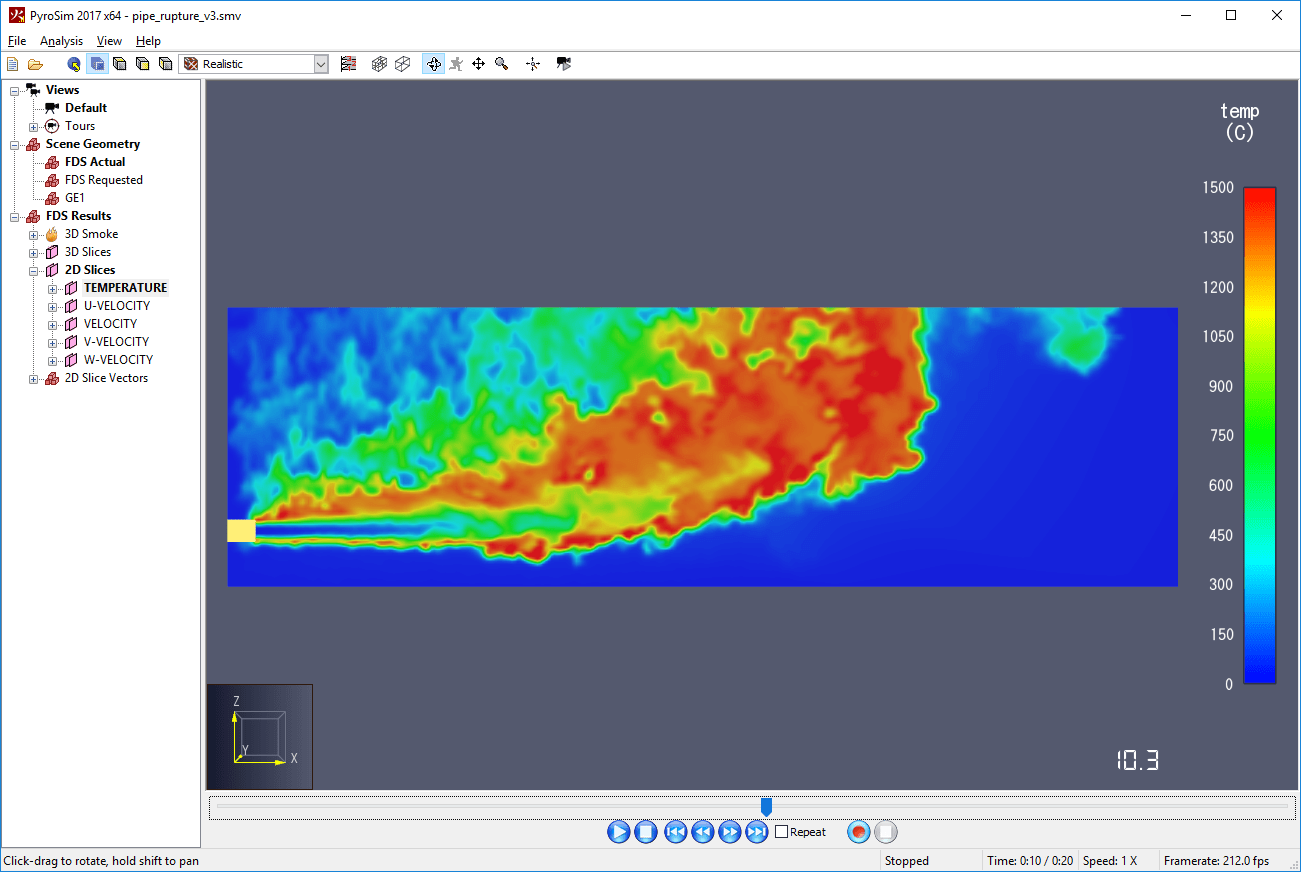
When an FDS simulation contains 2D slices, they will appear under the 2D Slices group in the Navigation View. The hierarchy appears in the Navigation View as FDS Results→2D Slices →Quantity→Slice Location→Mesh.
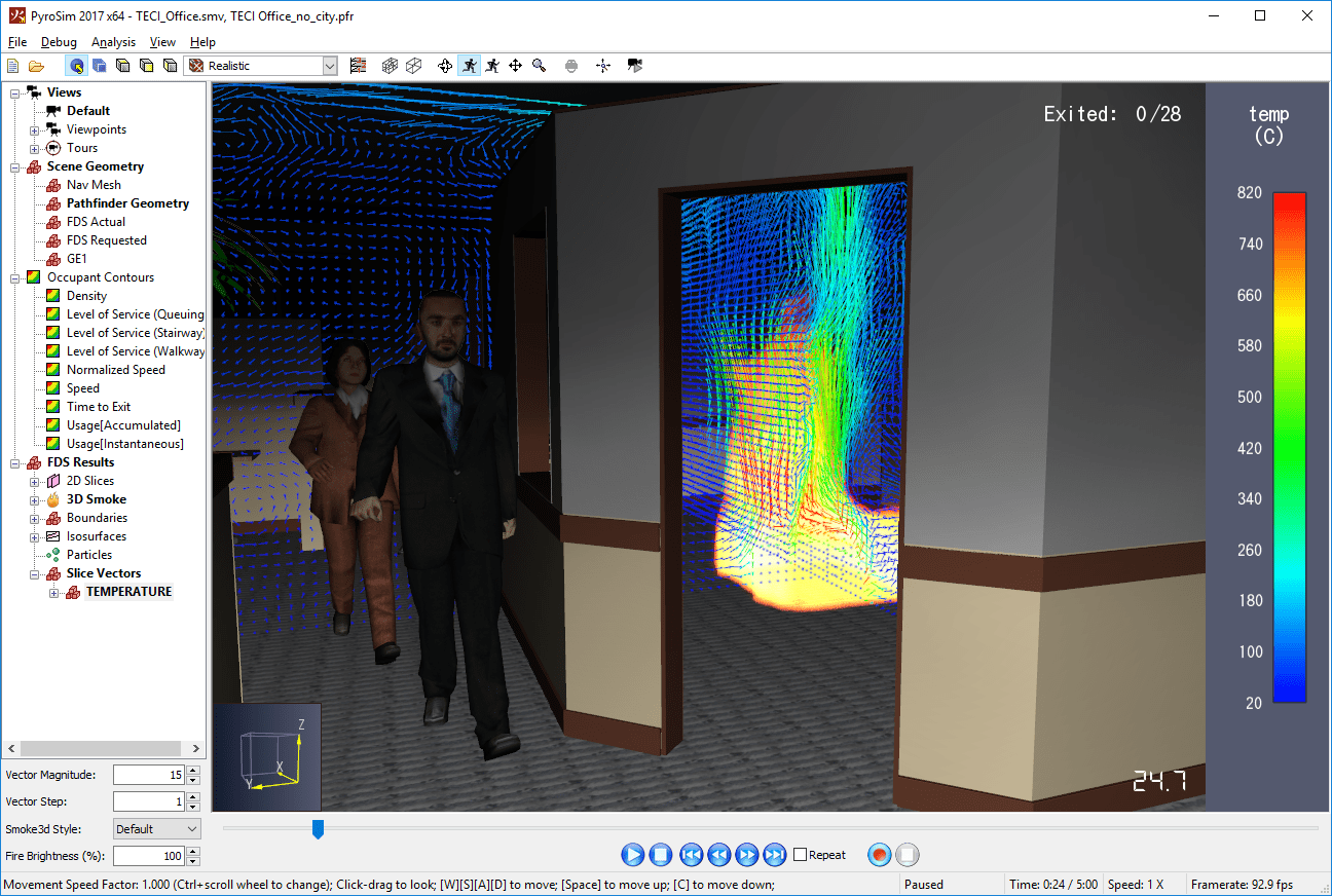
In FDS, 2D slices may optionally be created with the VECTORS option. When this option is enabled, FDS creates three additional 2D slice files containing the U,V,W coordinates of the air velocity. The Results application can combine these additional slice results to create 2D Slice Vectors.
2D Slice Vectors show the velocity of the air as vectors that point in the direction of the air flow and are scaled by the air speed. The velocity and color of each vector is determined at the center of the vector. Figure 79 shows 2D slice vectors that are colored by TEMPERATURE.
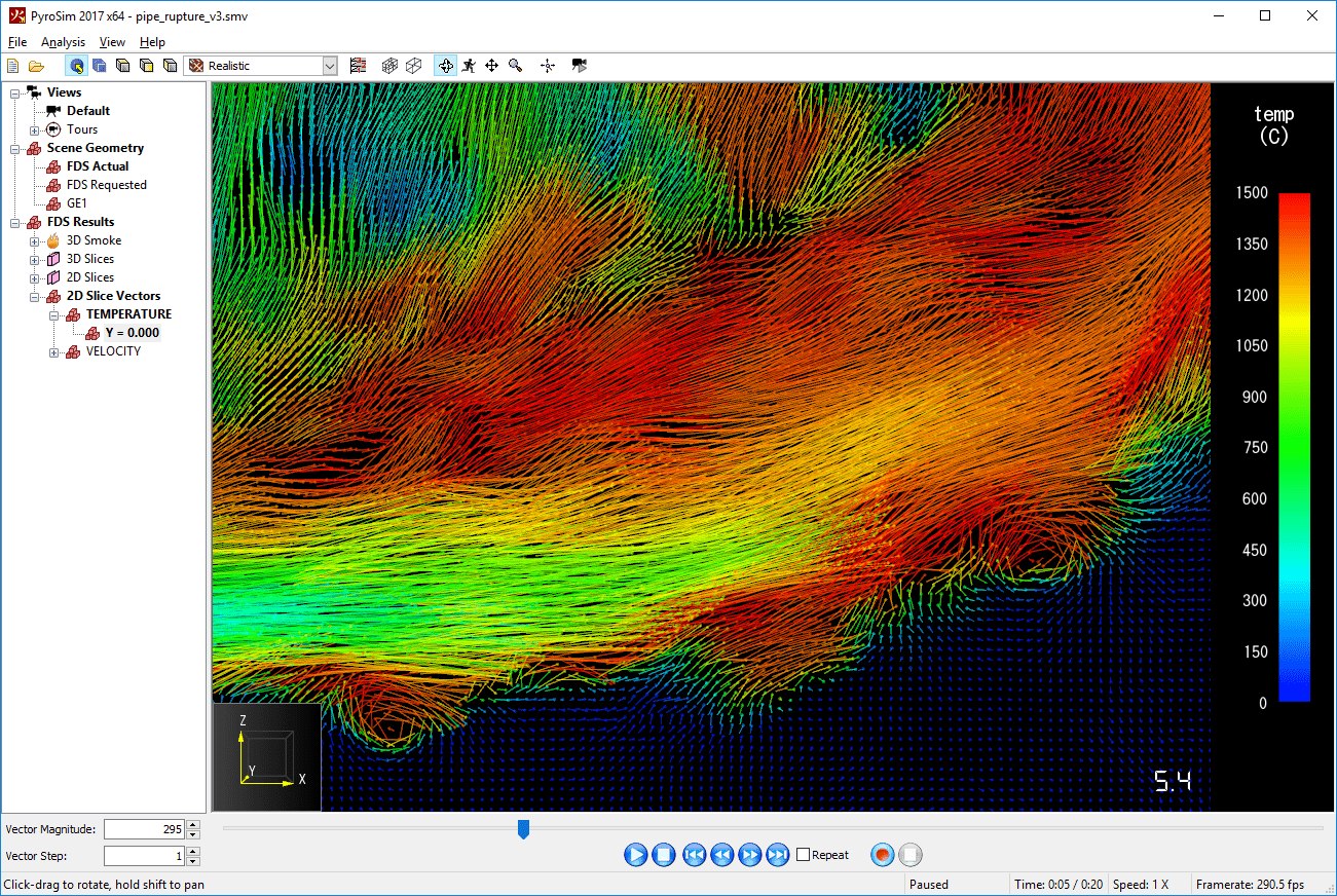
When an FDS simulation contains 2D slice vectors, they will appear under the 2D Slice Vectors group in the Navigation View. The hierarchy appears in the Navigation View as FDS Results→2D Slice Vectors →Quantity→Slice Location→Mesh.
To change the magnitude or density of the slice vectors, in the Navigation View, right-click the desired 2D slice vectors and click Properties. The Slice Vector Properties dialog will open as shown in Figure 80.
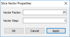
These options are also available in the Quick Settings when 2D slice vectors are active.
Boundaries show solid-phase and some gas-phase data at the boundaries of solid surfaces as shown in Figure 81.
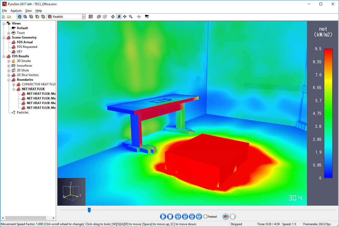
When an FDS simulation contains boundaries, they will appear under the Boundaries group in the Navigation View. The hierarchy appears in the Navigation View as FDS Results→Boundaries →Quantity→Mesh.
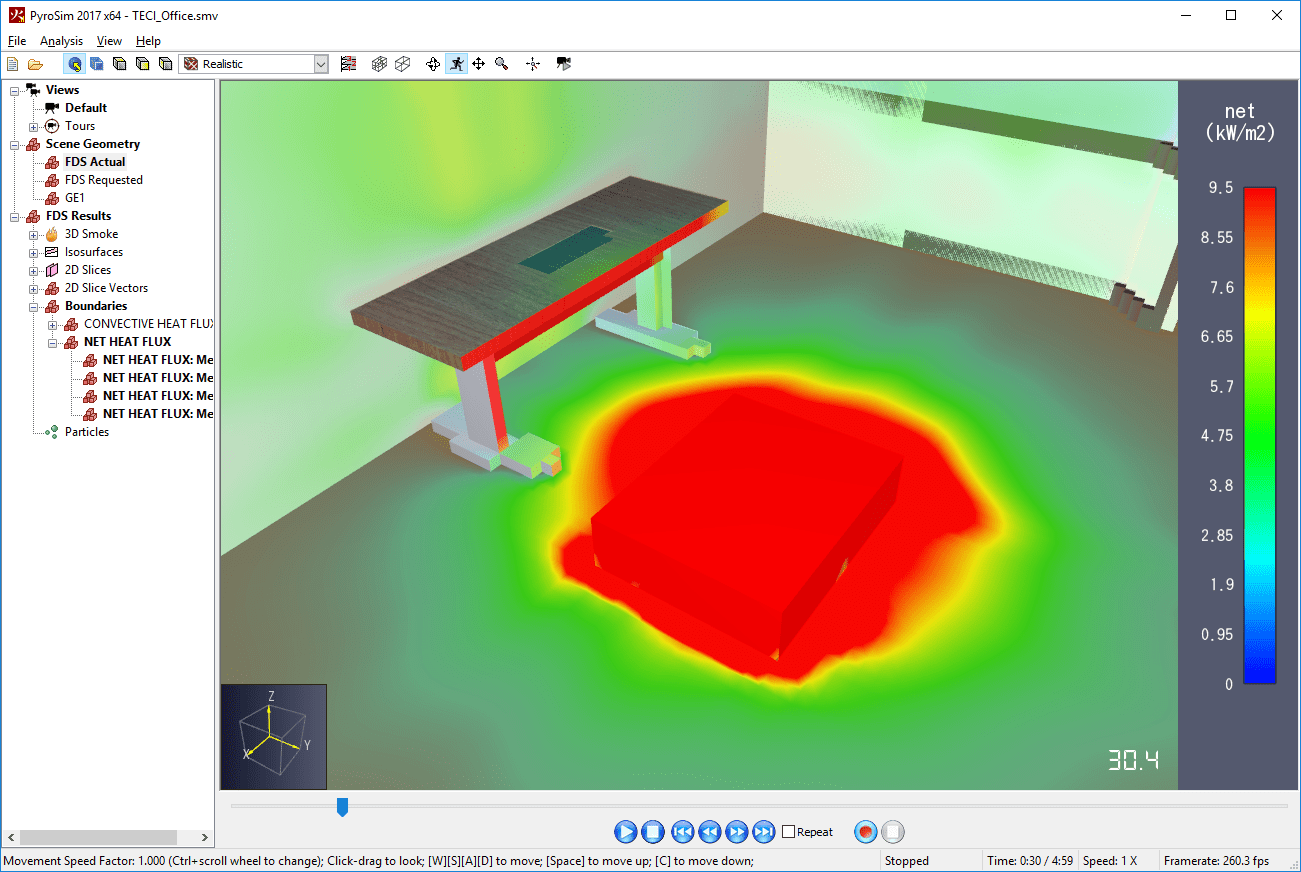
The colors of the boundaries are blended with those of the active geometry set. The amount of blending can be controlled with the Opacity setting in the FDS Preferences dialog (Global FDS Properties). The default opacity setting of 75% causes 75% of the color to come from the boundary and 25% from the geometry set. Setting this value to 100% would disable blending and only show the boundary colors. In addition, a gradient opacity function can be used to highlight specific boundary values as shown in Figure 82.
FDS supports the simulation of aerosol deposition, which can be used to track the deposition of various species on the boundaries of obstructions, such as soot gathering on walls and ceilings. FDS stores the output information in boundary files. By setting specific color parameters, the Results application can visualization soot deposition fairly realistically as shown in Figure 83.
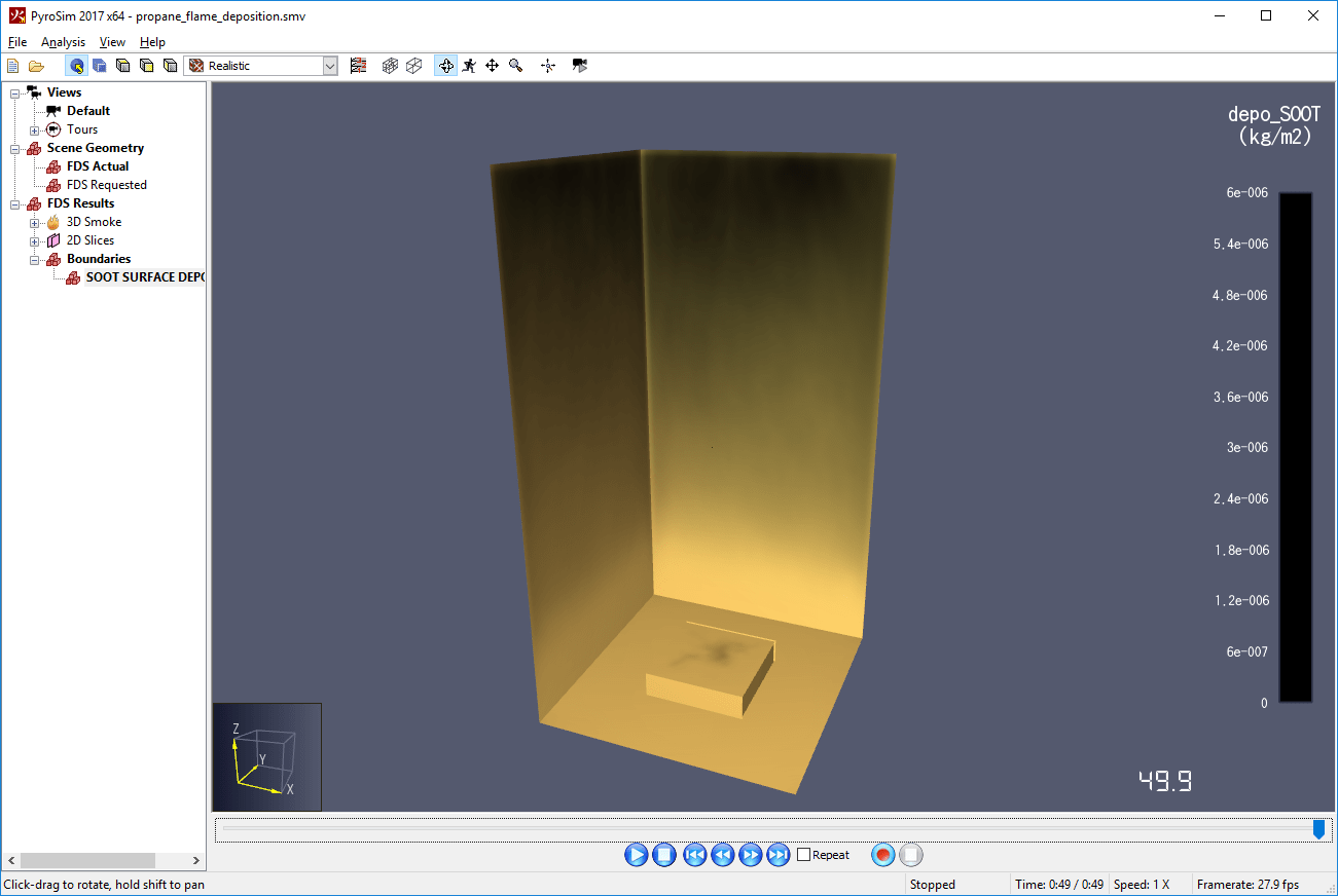
To recreate this visualization, perform the following:
FDS supports the injection of particles in a simulation. Particles can be used to trace air flow or to represent liquids, such as water or fuel. There can be several classes of particles in one simulation. Figure 84 shows tracer particles flowing through the model.
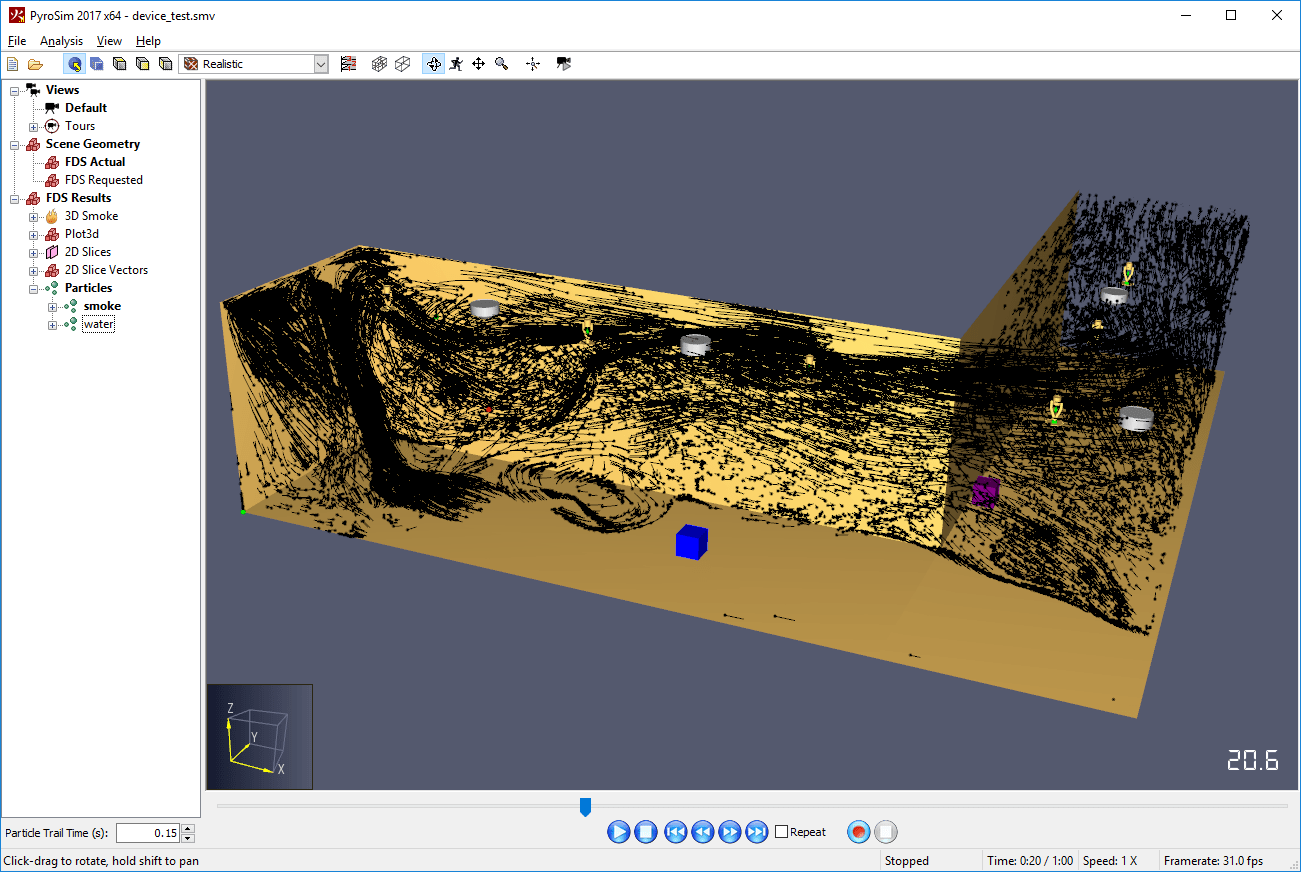
When an FDS simulation contains particles, they are found in the Navigation View and are organized as follows: FDS Results→Particles→Particle Class→Mesh.
By default, particles appear as dots and are a single color, but they may also be visualized with trails that show the particle motion. In addition, they may be colored by various particle quantities, if enabled in PyroSim or the FDS input file. To change the particle properties, in the Navigation View, right-click the desired particle class and select Properties. This will open the Particle Property Dialog as shown in Figure 85.
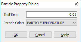
Controls the length of the particle trails by setting how far back in time in seconds to trace the path of the particle. If this value is zero, trails are turned off.
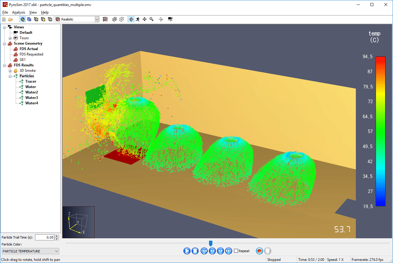
Controls the color of the particles. <Default> will color all the particles with a uniform color as specified in PyroSim or the FDS input file. Other values will cause a colorbar to appear and will color the particles individually according to their values. Figure 86 shows particles colored by their temperature.
Both the Trail Time and Particle Color may also be changed in the Quick Settings for the active particles.
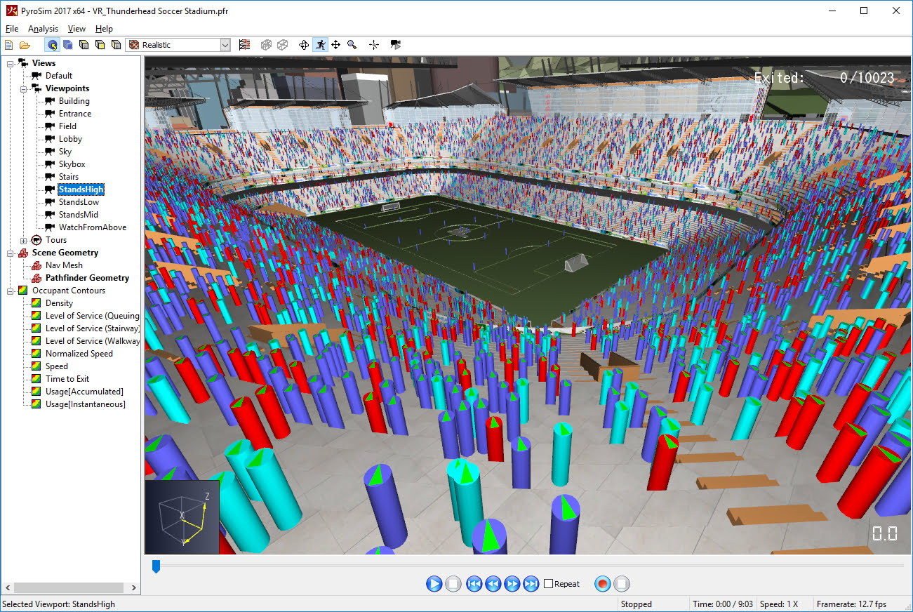
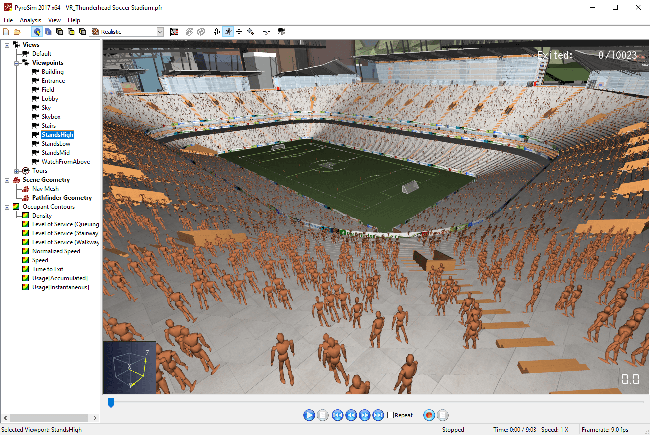
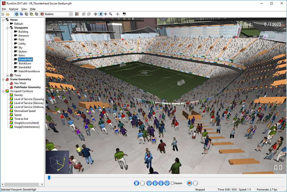
Occupants can be displayed in several ways. They can be shown as simple shapes, as realistic people, or as the artist’s wood mannequin as shown below.
All display options are found under the View→Occupant Display menu. Occupants can be displayed as follows:
 |  |
 |  |
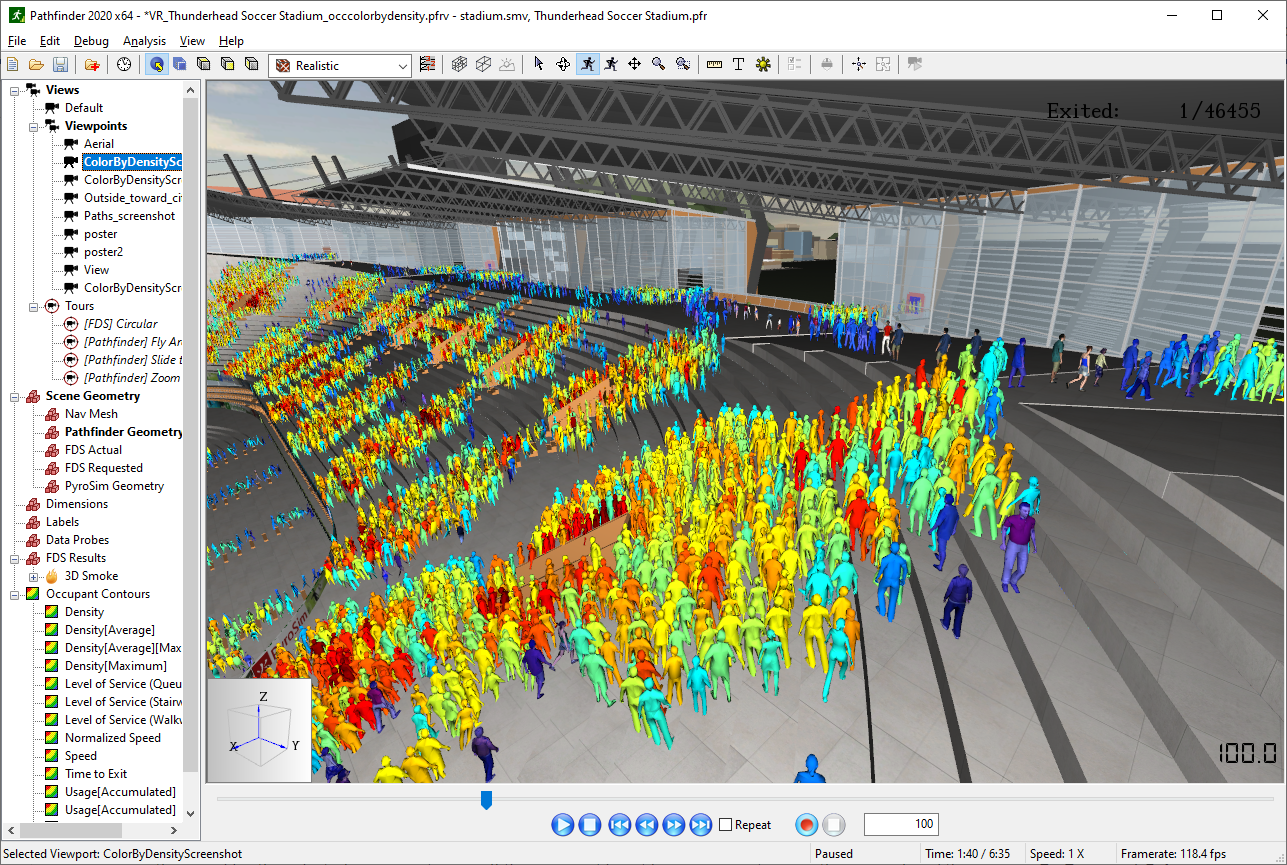
Occupants can be colored using several options found in the View→Occupant Color menu. In Figure 91, you can see occupants colored using a density occupant contour. Occupant coloring also affects the color of occupant paths, if enabled (see Viewing occupant paths).
The following options are available:
Colors the occupant according to the value of an occupant contour at the occupant’s location (see Occupant Contours/Heat Maps). Whenever this option is clicked, an occupant contour can be chosen from a list. The colorbar properties for this option are shared with the occupant contour itself. Any edits made to the occupant contour will reflect in the occupant colors as well, including colormap, highlight region, etc. If the colorbar’s opacity for a particular value is less than 100% and occupants are viewed as people, the occupant’s underlying texture will start to show through rather than making the occupant translucent. The more translucent the colorbar color is, the more the texture shows through. This effect can be seen in Figure 91, as the density contour coloring option in this case uses a feathered opacity.
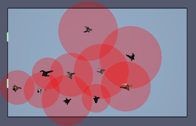
Occupant spacing disks visualize the amount of overlap per occupant for a specified radius. They are used in social distancing analysis. To show spacing disks for all occupants, on the View menu, point to Occupant Spacing Disks, and click Show All Spacing Disks. Alternatively, to only show spacing disks for selected occupants, click Show Selected Spacing Disks instead. Both of these options show the spacing disks at full-size, which may cause significant overlap of the disks. To reduce the amount of overlap, choose one of the Half-sized options from the Occupant Spacing Disks menu. This will cause the disks to display at half their size, which will reduce the overlap; however, this option should only be used if occupants have uniformly sized disks in each area. To turn off the display of spacing disks, click Hide Spacing Disks. Figure 92 shows an example of spacing disks generated from social distancing with a uniform distribution of radii.
To edit the size of the disks, on the View menu, point to Occupant Spacing Disks, and click Edit Spacing Disks. If social distancing is enabled in the Pathfinder model, the radius can be shown by selecting From Occupant Social Distancing in the Edit Spacing Disk dialog. Otherwise, a constant radius can be entered.
Occupants can be selected for tracking purposes by clicking on the occupant. When selected, the occupant and their path (if displayed) will turn yellow. Multiple occupants can be selected by holding CTRL when clicking them. They can be de-selected by clicking anywhere else in the model.
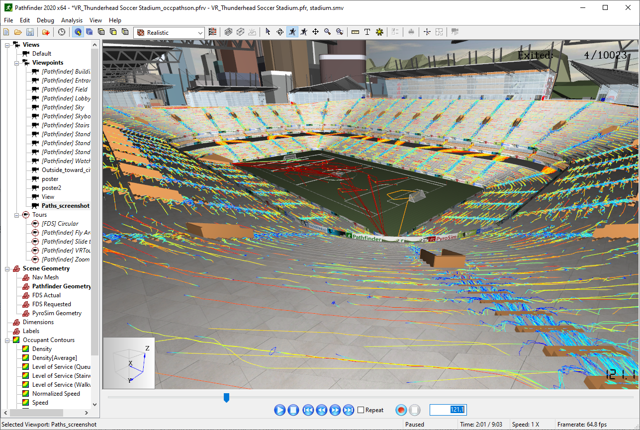
Occupant paths may be enabled to help visualize flow in an evacuation as shown in Figure 93. They can be shown by checking Show Occupant Paths in the View menu. When paths are enabled, each occupant’s path will be drawn from the time they entered the simulation to the current playing time. Paths are colored according to the current Occupant Color option as defined in Occupant Coloring. Each point on the path displays the color of the occupant when they were at that location, which allows a single path to have multiple colors. This can be seen in Figure 93 as the Occupant Color is set to By Occupant Speed.
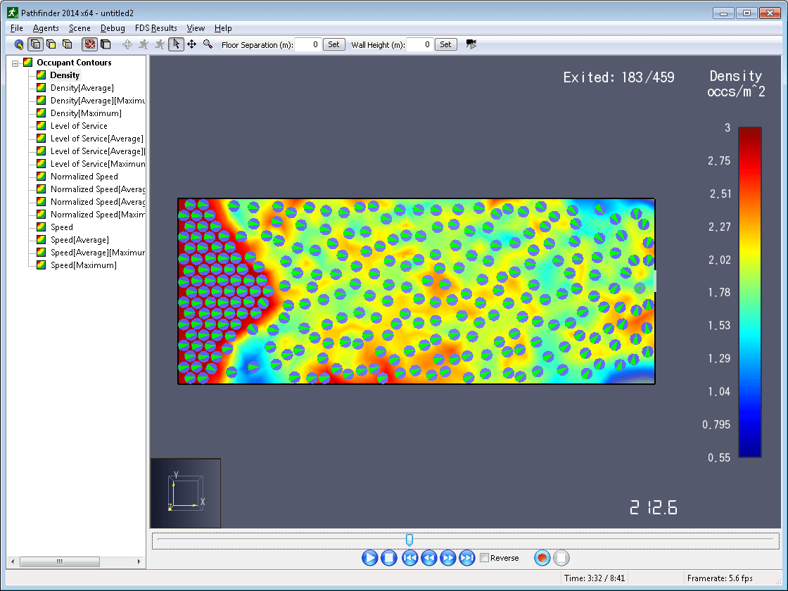
Pathfinder supports the visualization of dynamic occupant data on the floor areas of the model as shown in Figure 94. Referred to as occupant contours or heat maps, this animated data can give a qualitative visualization of the model’s performance.
Pathfinder supports the visualization of several types of occupant contours, including the following:
occupants/m2.Shows the amount of time it will take an occupant to exit from each point on the floor given the current playback time.
In addition to the basic contours, Pathfinder also provides the ability to filter any contour as follows:
30 s).
This can be useful for smoothing data over time and to act as a low-pass filter.unlimited).The ability to filter any contour gives the user a great deal of flexibility in visualizing contours. For instance, a contour could be created that displays the maximum average density. The averaging filter would act as a low-pass filter that reduces high-density peaks that may be short lived. The maximum filter would then be used to find the maximum of this smoothed data. This would be created by adding an average filter to the density contour and then adding a maximum filter to this averaging filter.
By default, a results file will contain several contours. More can be added or removed at any time.
Adding a contour can be done in one of two ways:
Performing either of these actions will open the New Occupant Contour dialog. In this dialog, select the desired contour quantity, and click OK. This will create the new contour and show its properties dialog as discussed below.
Contours can be removed at any time by selecting the desired contour in the navigation view, and either pressing DELETE on the keyboard or selecting Delete ![]() from the right-click menu.
from the right-click menu.
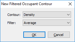
Contour filters can be added at any time in one of two ways:
This will show the New Filtered Occupant Contour dialog as shown in Figure 95. Select the desired properties and press OK to create the filter and show its properties dialog.
Contours can also be imported from older versions of the Results application (versions 2019.1.0515 and prior). This will import the list of available contours as well as their generation and visualization properties, but it will not import the contour data.
To import contours, under the File menu, select Import Occupant Contours.
In the file chooser dialog, choose the PFRMETA file that corresponds to the desired Pathfinder results file, and choose Open.
This will add the contours into the current results visualization.
Contours can also be duplicated. This is useful for creating several versions of a particular quantity, such as showing different averaging intervals or creating several snapshots of a contour at different times.
To duplicate a contour, in the navigation view, right-click the contour and select Duplicate. This will create and add a duplicate of the selected contour. Several contours may be duplicated at once by selecting several in the tree before duplicating.
There are several global properties that control how each contour is generated and displayed.
To modify these properties, right-click the "Occupant Contours" group in the navigation view as shown in Figure 96, and select Properties.
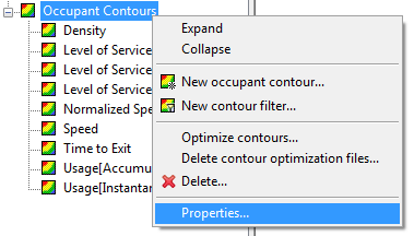
This will show the Occupant Contours Properties dialog as shown in Figure 97.
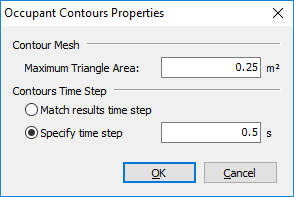
Allows the contour time step to be specified. Values higher than the time step of the Pathfinder results will decrease the time accuracy of the generated contours but will also decrease the calculation time and disk space requirements for the contour files. The specified time step will be rounded to the nearest multiple of the Pathfinder results time step.
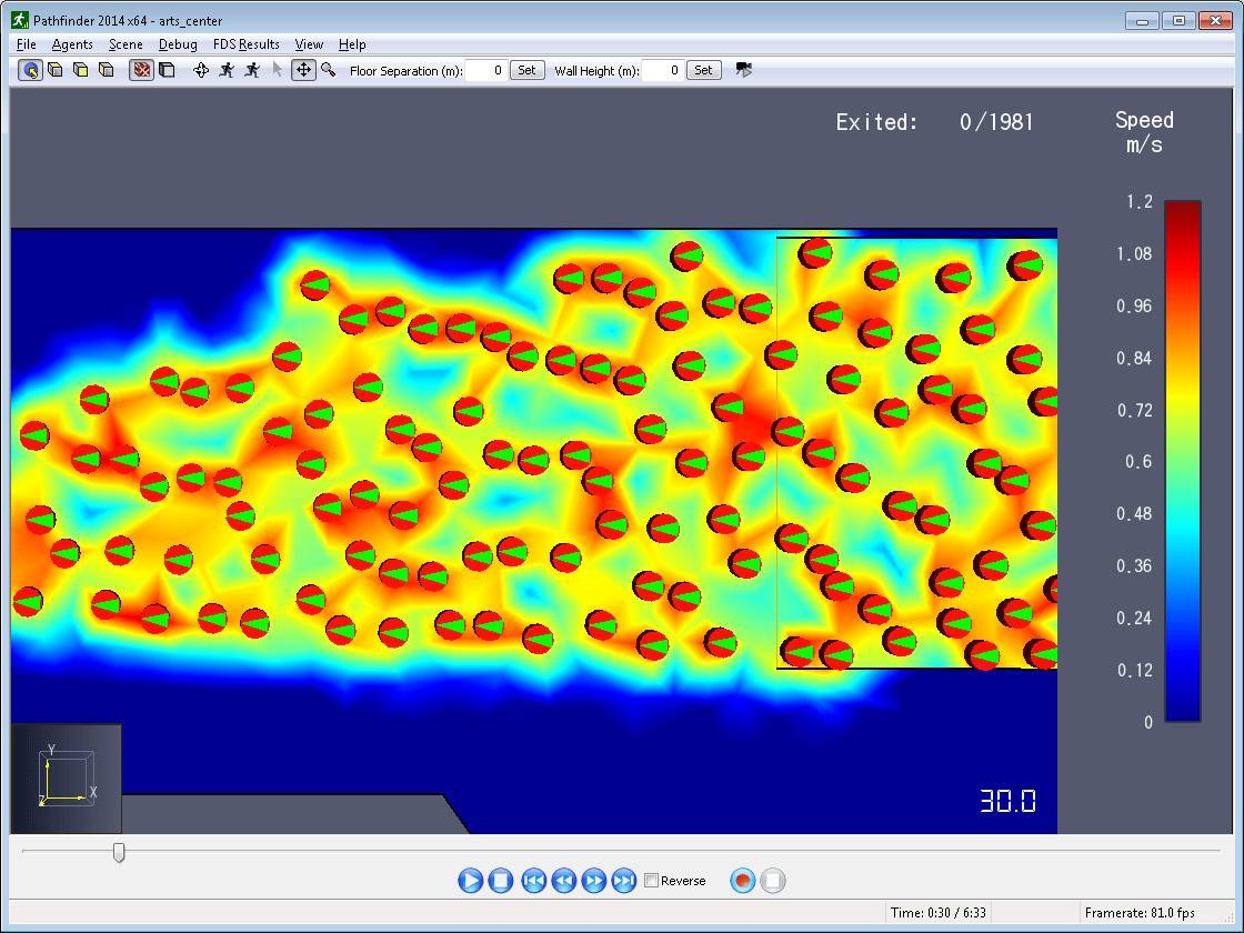 | 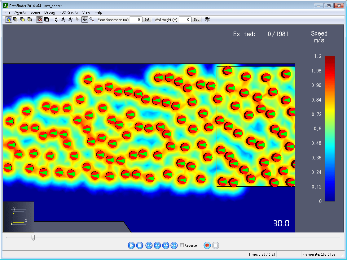 |
Each contour also contains a set of properties that control the generation of the contour as well as its visualization. To set the properties of a contour, right-click the contour in the navigation view and select Properties. This will show the properties dialog for that contour.
Each contour has a potentially different set of properties. The properties dialog for density is shown in Figure 100.
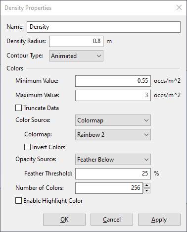
The following is composite list of all contour properties that control the creation of the contours:
30 s is entered for an average density contour, the average will only be calculated for the trailing 30 seconds of density data at each time step.
So at t=120s, the average is calculated over the time range of [90,120] s.
If this option is left unchecked, the calculation will take place over the entire time range preceding each time step.
So at t=120s, the time range would be [0,120] s.400 s of results data available, the time interval will be [0,400] s.In addition to the above properties, colorbar settings can also be specified as described in Colorbars with the following additional considerations:
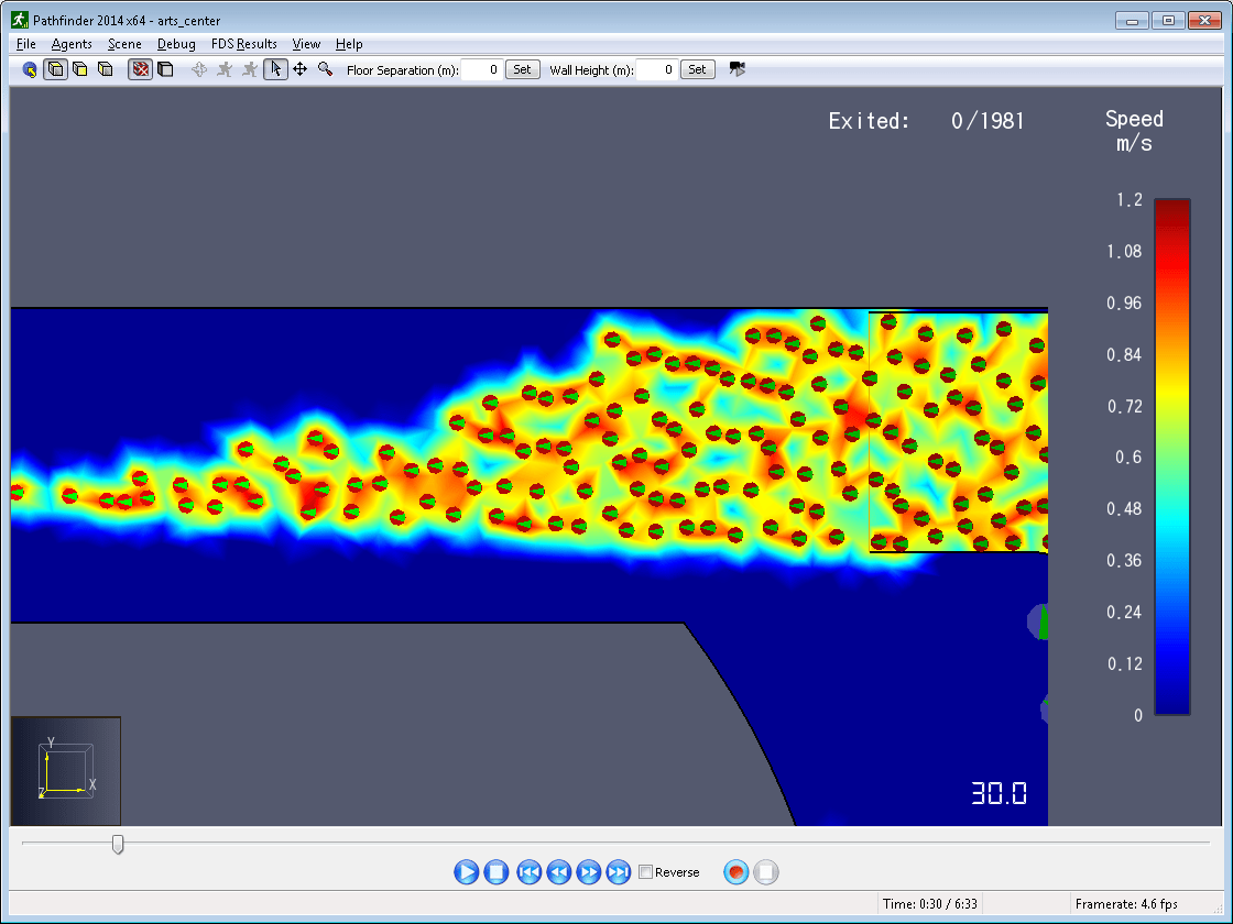 |  |
One contour may be activated/shown at a time. To activate a contour, either double-click it in the navigation view, or right-click it and select Show from the context menu. The first time this is performed, a dialog will appear asking whether to optimize the contour. Choosing Yes will cause a progress bar to appear while the contour is optimized and stored in an optimization file.
See Optimizing Contours below for more information about optimization. Check Remember my decision to prevent being asked in the future. This can be changed in the preferences by going to File→Preferences.
Once a contour is active, it will appear bold in the navigation view. In the model view, the contour will appear overlaid on the navigation mesh or imported geometry and a colorbar legend will appear to the right.
The active contour can be hidden by either double-clicking it in the navigation view or right-clicking it and selecting Hide.
Each contour may optionally be optimized for playback. Optimizing a contour is especially helpful with complex models, as it typically allows for much smoother playback and faster seeking when the contour is active, especially for contour filters. Contour optimization only has to be performed once per contour, as the optimization is stored on disk, allowing it to be accessed during later sessions.
The optimization file for each contour is stored in the same directory as the results and will have a filename based on the results filename and the contour’s quantity and filter.
For instance, a model named test.pth will have a density file name test_density.octranim.
There are several ways to optimize a contour. The first two methods optimize the contour ahead of time. This is the best option, but it comes at the cost of requiring time up-front to calculate the contour.
Here are all the options for optimizing a contour:
Contours can be optimized manually by right-clicking the contours to optimize in the navigation view and selecting *Optimize * from the context menu.
If a contour has not been optimized using one of the two previous options, contours may instead be optimized dynamically during playback and while seeking. To enable this option, open the preferences dialog as described previously, and check the box next to Enable dynamic optimization. This will cause the contour frames to be optimized as requested either during playback or during seeking of Pathfinder results. Once a frame of contour data has been optimized and saved to disk, it will be retrieved from disk whenever that frame is needed again.
Once a contour has been optimized, there are some actions that may cause the optimization to become invalid. Pathfinder will re-optimize if necessary when the user requests that it be optimized again using one of the above methods.
The following actions may cause a contour optimization to become invalid:
Contour optimization files may be very large for models with large navigation areas and/or long simulation times. These optimization files may be deleted at any time to preserve disk space in one of two ways:
When using the Level of Service (LOS) contour, the colors are defined as follows:
| Color - LOS | Walking | Queueing | Stairs |
|---|---|---|---|
| 35 ft2 (3.3 m2) per person or greater | 13 ft2 (1.2 m2) per person or greater | 20 ft2 (1.9 m2) per person or greater | |
| 25 ft2 (2.3 m2)-35 ft2 per person | 10 ft2 (.93 m2)-13 ft2 per person | 15 ft2 (1.4 m2)-20 ft2 per person | |
| 15 ft2 (1.4 m2)-25 ft2 per person | 7 ft2 (.65 m2)-10 ft2 per person | 10 ft2 (.93 m2)-15 ft2 per person | |
| 10 ft2 (0.93 m2)-15 ft2 per person | 3 ft2 (0.28 m2)-7 ft2 per person | 7 ft2 (0.65 m2)-10 ft2 per person | |
| 5 ft2 (0.46 m2)-10 ft2 per person | 2 ft2 (0.19 m2)-3 ft2 per person | 4 ft2 (0.37 m2)-7 ft2 per person | |
| 5 ft2 (0.46 m2) per person or less | 2 ft2 (0.19 m2) per person or less | 4 ft2 (0.37 m2) per person or less |
Sample points can be created from occupant contours, which can be used to export time-series data and show plot from the contour as explained in Exporting Data and Time History Plots. In order to create a sample point, perform the following steps:
Sample points are listed under the Sample Points group of the Navigation View. From there they be renamed and deleted. They can also be hidden from view by clicking on the View menu and unchecking Show Sample Points.
Pathfinder and FDS output several data files, including many CSV (comma-separated value) files. CSV files are convenient for storing tabular data arranged in rows and columns in a human-readable format. Many of these output files from Pathfinder and FDS contain data for various objects over time. For instance, the FDS hrr.csv output file contains information about the burner’s heat release rate over time, among other quantities.
These CSV output files can be loaded and plotted within the Results application. A link to the CSV file is saved with the visualization file so it can be loaded again the next time the visualization file is loaded.
Results supports most of the CSV output files from FDS and Pathfinder. It can also load other CSV files, however, as long as they contain the following:
While not required, it is also recommended that the CSV file specifies the following:
width or density.
For instance, there can be multiple columns with a description of Door01.
These would be differentiated by a quantity in each one, such as width, flowrate, etc.
The quantity can either be in its own header row or it can be combined with the description row.
If it is combined with the description row, it must be in this format:
description_quantity, where description is the description of the column, such as Door01, and quantity is the quantity for the column, such as width.m or kg/s.
The unit can either be in its own header row or it can be combined with either the description row or the quantity row.
If it is combined with the description or quantity, the unit must be specified at the end and be in parenthesis.
For instance, if it is combined with both, it would be formatted as: Door01_width (m).
In this example, the description is Door01, the quantity is width, and the unit is m.The following are examples of valid CSV headers:
s,   kW, kW,    kW,    kW,    ...
Time,HRR,Q_RADI,Q_CONV,Q_COND,...
Time,Region00,Region00,Region01,Region01,...
Time,Density, Velocity,Density, Velocity,...
s,   pers/m2, m/s,     pers/m2, m/s,     ...
Time (s),Door01_Flowrate (occs/s),Door01_Width (m), ...
To load a CSV file into Results, perform the following:
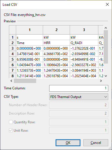
The Load CSV Dialog shows a preview of the CSV file, which includes the first 10 rows and 20 columns. The following can be entered in the dialog:
<custom>.
If <custom> is selected, the rest of the fields in the Load CSV Dialog must be specified.CSV files are managed in the Navigation View.
When a CSV file is loaded into Results, it will be added to the Results as a CSV File object.
The CSV File object will appear under the XY Plot Data group in the Navigation View as shown in Figure 104.
Each non-time column in the CSV File will be added to the Results as a Time Series object and will appear under the CSV File object in the Navigation View.
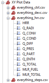
Individual Time Series objects can be deleted from the CSV File by selecting the item and pressing Delete. The entire CSV File can be deleted by selecting it and pressing Delete.
When the visualization file is saved, a relative path to the CSV file is also saved. When the visualization file is loaded, the path to the CSV file is reconstructed by appending the saved relative path to the current visualization file’s directory.
When results are refreshed (see Refreshing Results), the Results application will check for any changes to the columns in the CSV file. If any columns have been added or removed, Time Series objects will also be added or removed from the CSV File object. If any columns have changed order, Results will also correctly track their new positions as long as their name, quantity, and unit stay the same.
Time Series objects from CSV files can be exported or plotted within Results. See Exporting Data and Time History Plots for more information.
The Results application allows time series data to be exported to a CSV (comma-separated value) or TSV (tab-separated value) file. Currently, data can be exported from the following objects:
In order to export the data:
The data for the selected objects will be written to the file. The first column will always be the time, and each subsequent column will be the data for each selected object. The time resolution for the file is based on the underlying time step size of the objects. For instance, if exporting data for occupant contour sample points, the time step size in the CSV file will be the same as the time step specified for the contours as described in Global Contour Properties. For Data3D Points, it depends on the output time step of the FDS simulation. For CSV Time Series objects, it depends on the time stamps in the CSV file. When combining points from multiple sources, the times listed in the CSV file will be the union of the keyframes from all the sources. This might result in time-interpolated data for some of the points.
The Results application allows time history data to be displayed in a plot. Currently, data can be shown from following objects:
In order to show the plot data:
This will display the Time History Plots dialog, as shown in Figure 105. Alternatively, double-click the desired plot from the Navigation View to show the plot.
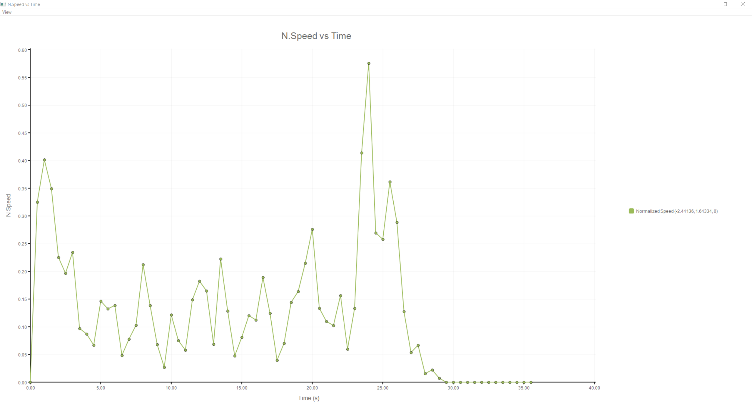
To create a screenshot of the plot, on the File menu, click Save Screenshot or press F11. Enter the desired screenshot name and click OK to create the screenshot.
To change how the plot data is displayed, use the View menu. The following options are available:
The Results application provides some post-processing capabilities, including the ability to generate contours that show dynamic occupant data overlaid on the navigation mesh or imported geometry as shown in Figure 106.
Contours can either be calculated as results are played back or can be optimized and stored on disk for later retrieval. Optimization is discussed further in the User Manual. The calculation of the contours is described in this guide.
Contours are calculated using a sub-divided version of the navigation mesh as seen in Figure 108.
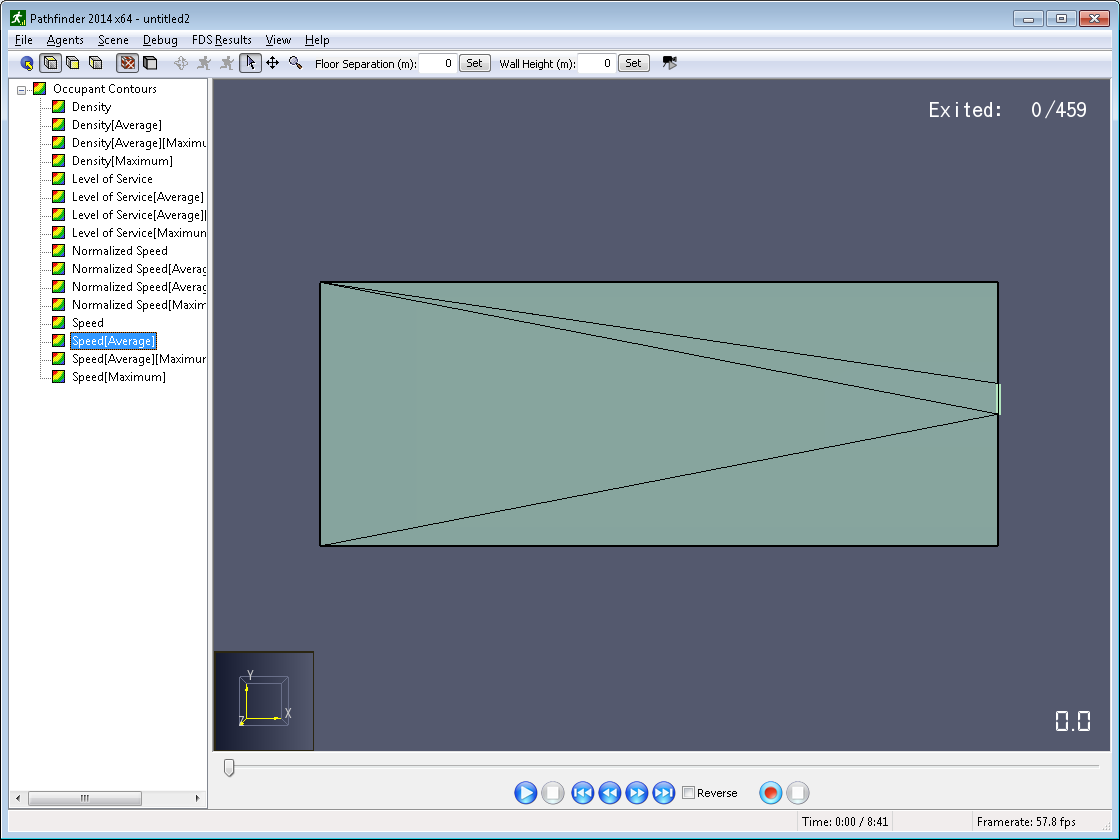 | 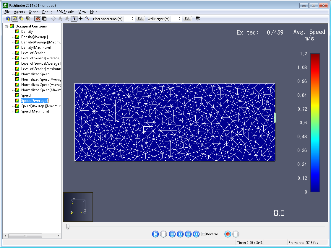 |
Contour values are calculated at the vertices of the triangles in the contour mesh and are linearly interpolated across triangles to produce the shading. The contour mesh is used only to display occupant contours and is independent from the navigation mesh used during the simulation. The spatial resolution of the contour mesh as well as the update frequency can be controlled using the Occupant Contours Properties dialog. Smaller values for space and time resolution offer smoother contours at the cost of greater calculation time and memory requirements.
Frames of contour data are produced throughout time depending on both the Pathfinder results data frames and the time step specified in the Occupant Contours Properties dialog as discussed in the User Manual. Each contour frame lines up in time with a frame of occupant animation data, though there does not have to be a one-to-one correspondence. This ensures that contour data is only produced when occupants are at known positions rather than interpolated positions. To view contour data at times between contour frames, the data is linearly interpolated between frames.
The density calculated at each vertex of the contour mesh is dependent on the location of nearby occupants and the value of the Density Radius parameter. Any occupant intersecting the circle around a vertex contributes to the density at that vertex. Occupants who partially fall within the circle around a vertex contribute partially based on intersection area.
Increasing the Density Radius parameter smooths out contours by eliminating peaks and valleys in the density calculation. This effect will tend to be more visible near the edges of dense flows and more stable within uniformly dense regions due to partial attribution of occupants intersected by the density measurement radius.
The following steps describe in detail how the density values that control contour colors are calculated.
Level of Service is implemented the same as density but with three special color maps. Each color map represents a different type of terrain, including Walkway, Stairway, and Queuing (Fruin and Strakosch 1987).
For each occupant, their speed is applied to the vertices of the contour mesh within a distance of ri (Influence Radius in the User Manual). The speed value at each vertex is calculated as follows:
The normalized speed contour is calculated similarly to the speed contour, except that the speed value per vertex is the following:
Where sxmax is the maximum speed of occupant x.
The usage value at each vertex is calculated as follows:
The accumulated usage contour is implemented as a time-integrated filter on top of an instantaneous usage contour. See Integrate for more information about the integration filter.
The Time to Exit contour value at each vertex is calculated as follows:
Where texit is the occupant’s exit time and tcurr is the current contour calculation time.
Average contours are applied on top of other contours.
They are calculated over a user-specified interval that is always trailing a particular time step.
So if the averaging interval is 30 s long, then at t=120 s, the averaging interval is [90,120] s.
The interval cannot go back in time, however, so at t=10 s, the interval is [0,10] s.
For each vertex, the vertex contour values of the base contour are averaged over this interval to produce the final vertex value as follows:
Where x is the index of the contour frame for the current time step, n is the number of frames that intersect the calculation interval, vf is the vertex value of the base contour at frame f.
Maximum contours are applied similarly to average contours. For each vertex, the final vertex value is the maximum of the vertex values of the base contour over the time interval as follows:
Currently, the integration filter is not exposed as a general contour filter - it is only available incorporated into the accumulated usage contour. The integration filter is implemented on a per-vertex basis as follows:
Where tf is the time of frame f, and tf-1 is the time at frame f-1.
The floating license server provides an administration web service that can assist with diagnosing many floating license problems. If the license server is installed on the local machine, the license administration server can be accessed at the following web address: http://localhost:5054
If the license server is installed on a remote machine, replace localhost with the name of the remote machine (i.e. the host name of the floating license server).
Once you have opened the Reprise License Server Administration page, you can use the Status commands to attempt to debug the license server problem yourself, or you can send a diagnostic report to support@thunderheadeng.com for assistance.
To generate a diagnostic report:
rlmdiag.txt) to support@thunderheadeng.comThe Results application utilizes several advanced graphics card features in order to provide accelerated display of results. If you experience crashes or problems with display, you should first make sure your video card drivers are up-to-date. If they are, there may be some rendering options that can be turned off in the preferences at the expense of decreased fidelity or rendering speed.
If you encounter these problems, please let us know the make/model of your video card and what video driver you are using. This will help us improve our software and increase compatibility.
If the Results application immediately closes when first started, this is usually the result of bugs in the graphics driver. First make sure you are using the latest drivers for you graphics hardware. Some computers may have two graphics adapters, especially laptops. If you are not sure which graphics are being used for the Results application, update the drivers for both GPUs. If this still doesn’t fix the problem, try running the Results in safe-mode.
This can be done as follows:
PathfinderResults.exe.
This executable is found in the install folder for Pathfinder.-safemode.Running the results in safe-mode will disable several advanced graphics features. It will also show a console window with some logging information.
If the Results application starts successfully in safe-mode, the graphics features can be re-enabled one at a time in the Preferences dialog to see which one caused the problem, see Controlling Drawing Detail/Speed.
If the Results application crashes when specific results are loaded, such as FDS smoke and fire, the graphics card drivers are usually at fault. First try updating the graphics drivers. If that does not fix the problem, try using a compatibility setting for the result type being loaded. For more information, see Controlling Drawing Detail/Speed.
If particular results do not display correctly, such as a 2D slice that never changes color, this is usually an issue with the graphics card drivers. Older Intel HD Graphics drivers are especially problematic. First try updating the graphics drivers. If that does not fix the problem, try using a compatibility setting for the result type being displayed. For more information, see Controlling Drawing Detail/Speed.
If FDS results, such as fire and smoke, stutter or pause frequently during playback, this may be because the results files are too large to stream. See File Streaming for more information on combatting this problem.
When results are streaming from disk (File Streaming), they require a connection to the file on disk. If the result files are on a remote machine, there is a possibility that the files can become disconnected from the Results application. In this case, the application may become frozen as it tries to read more data from the disconnected disk. This is usually caused by stability issues with the network.
The current remedy for this problem is to copy the results to the local machine to ensure a more reliable connection with the Results application.
There are some known issues with the Results. Some of these issues may be fixed in future releases, while others may be deemed non-critical with no plan for a fix.
smoke_test problem presented in Chapter 3 of the Smokeview Verification Guide (Forney 2019), only the Use Hardware Shaders render method for smoke produces the expected greyscale values when viewing the scene from the front camera.
See Controlling Drawing Detail/Speed for more information on the render method.
This is because the other modes draw one smoke slice too many, making the smoke appear slightly too opaque.
The extra slice is drawn because the obstructions line up exactly with some of the slice planes, and the scene geometry is drawn slightly offset away from the camera using polygon offset to allow some objects to appear on top of the obstructions without interference artifacts.
When viewed from any perspective other than the front, the greyscale values should be correct in these modes.If you need assistance, or wish to provide feedback about any of our products, contact support@thunderheadeng.com
Forney, Glenn. 2019. Smokeview, A Tool for Visualizing Fire Dynamics Simulation Data Volume II: Technical Reference Guide, NIST Special Publication 1017-2. Sixth Edition. National Institute of Standards and Technology, Gaithersburg, Maryland, USA: NIST.
———. 2019. Smokeview, A Tool for Visualizing Fire Dynamics Simulation Data Volume III: Verification Guide, NIST Special Publication 1017-3. Sixth Edition. National Institute of Standards and Technology, Gaithersburg, Maryland, USA: NIST.
Fruin, J.J., and G.R. Strakosch. 1987. Pedestrian Planning and Design. Elevator World. https://books.google.com/books?id=vrckAQAAMAAJ.