 1.55 ± 0.18 m/s. | 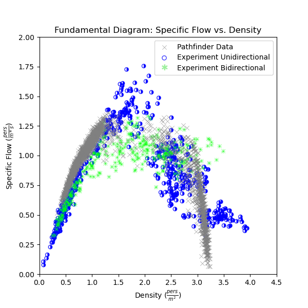 1.55 ± 0.18 m/s. |
Verification and Validation for Pathfinder
There is a newer version of this document. To view the latest version, click here.
Thunderhead Engineering makes no warranty, expressed or implied, to users of Pathfinder, and accepts no responsibility for its use. Users of Pathfinder assume sole responsibility under Federal law for determining the appropriateness of its use in any particular application; for any conclusions drawn from the results of its use; and for any actions taken or not taken as a result of analyses performed using these tools.
Users are warned that Pathfinder is intended for use only by those competent in the field of pedestrian modeling. Pathfinder is intended only to supplement the informed judgment of the qualified user. The software package is a computer model that may or may not have predictive capability when applied to a specific set of factual circumstances. Lack of accurate predictions by the model could lead to erroneous conclusions. All results should be evaluated by an informed user.
This document presents verification and validation test data for the Pathfinder simulator.
The following definitions are used throughout this document:
Usage of the terms Verification and Validation in this document is consistent with the terminology presented in IEEE Standard 1012 (“IEEE 1012-2016 - IEEE Standard for System, Software, and Hardware Verification and Validation” 2016) and ISO 16730-1 (“ISO 16730-1:2015E - Fire Safety Engineering — Procedures and Requirements for Verification and Validation of Calculation Methods” 2015).
Most test cases in this chapter are executed using three different configurations (modes) based on the Behavior Mode option and the Limit Door Flow Rate option in Pathfinder’s Simulation Parameters dialog.
In each case, all other simulator options are left at the default setting unless otherwise specified. For cases that examine speed-density behavior, only the Steering mode is applicable.
The SFPE mode supported by Pathfinder allows occupants to instantly transition between speeds without accounting for acceleration. However, when predicting the results for simulations run using the Steering mode, it is necessary to account for inertia.
Assuming an occupant must travel some distance \(d\), this is generally done in the following way:
1.1 seconds.
\(v_{0}\) is generally zero and \(v_{1}\) is the occupant’s maximum velocity.0.0 m/s and walk distance \(d\) is then given by: \(t = t_{1} + t_{2}\).Inertia also impacts the effective flow rates through the doors for the Steering+SFPE mode, since each occupant must accelerate when released to pass through the door.
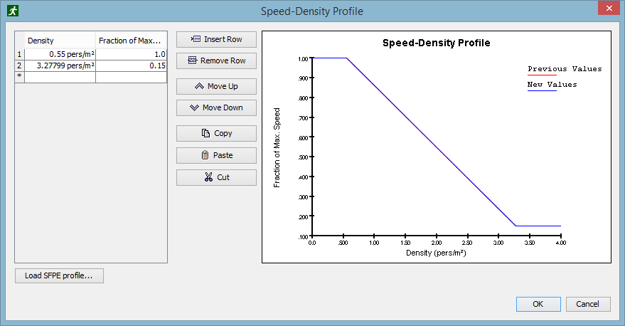
In Pathfinder, the user can specify a Speed-Density Profile - the fundamental diagram.
Since occupants can have different individual walking speeds, the user defines a normalized profile.
The speed-density profile for that occupant is obtained by multiplying that occupant’s speed by the normalized speed-density profile (Figure 1).
The default normalized speed-density profile corresponds to the SFPE specification (SFPE 2019) with the modification that, at high densities, the speed goes to a factor of 0.15 rather than zero.
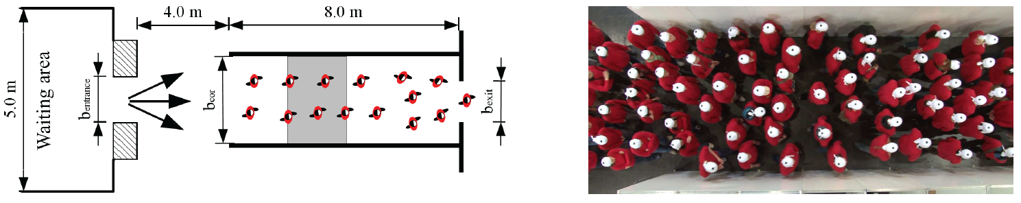
"Transitions in pedestrian fundamental diagrams of straight corridors and T-junctions" (Zhang et al. 2011), "Ordering in bidirectional pedestrian flows and its influence on the fundamental diagram" (Zhang et al. 2011) and "Empirical Characteristics of Different Types of Pedestrian Streams" (Zhang and Seyfried 2013) describe a series of experiments in which they measured the fundamental diagram by controlling density in a corridor by varying the entrance and exit widths (Figure 2).
You can download the actual experimental videos and supporting documentation from the Pedestrian Dynamics Data Archive.
This validation case will focus on the unidirectional flow results.
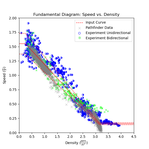
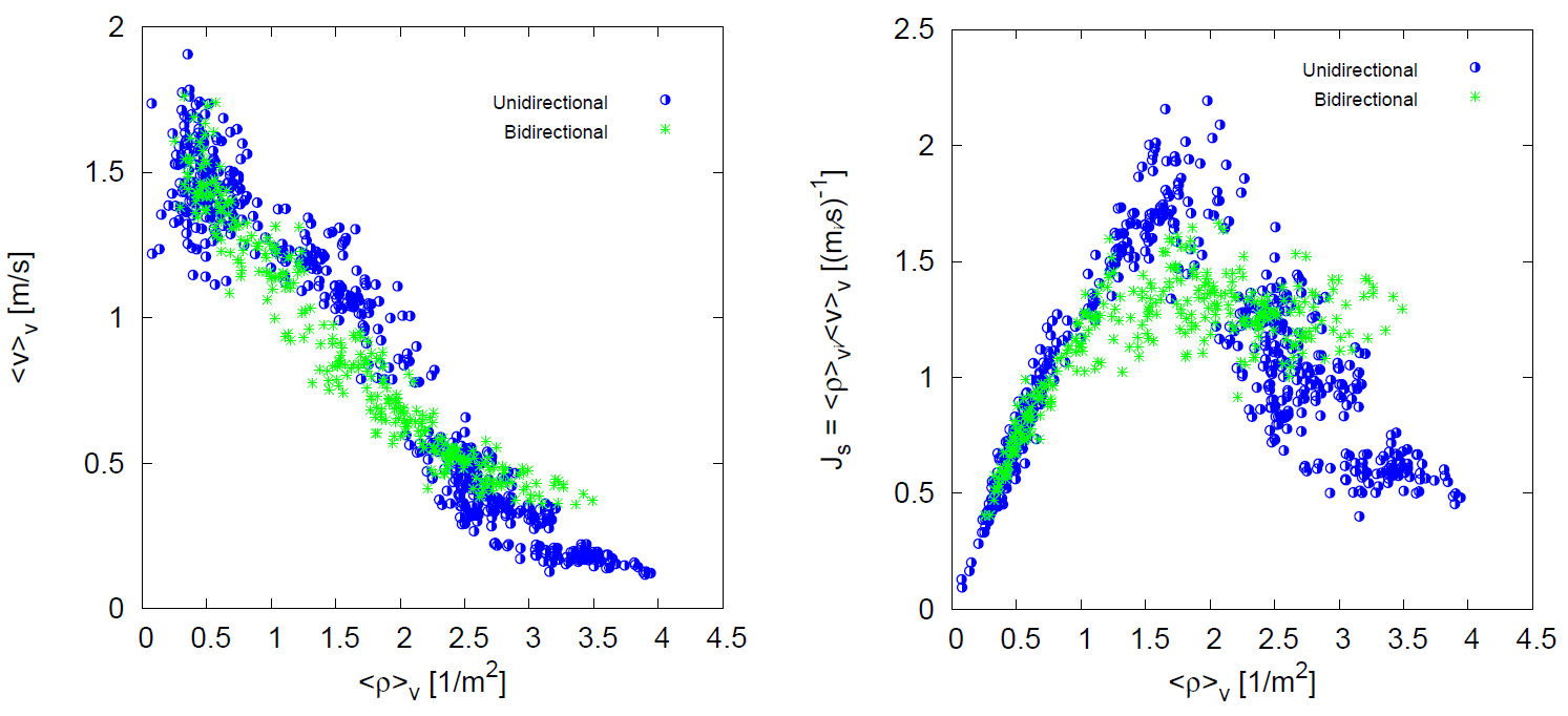
A summary of the experimental results for unidirectional and bidirectional flows is shown in Figure 3.
The corresponding SFPE specification curves are shown in Figure 4.
Compared to the SFPE calculations, the Zhang and Seyfried experiments have a higher occupant speed (measured free velocity of 1.55 ± 0.18 m/s) and a significantly higher measured specific flow (although the paper notes large specific flow variations for small changes in the experimental setup for densities greater than 2 pers/m2).
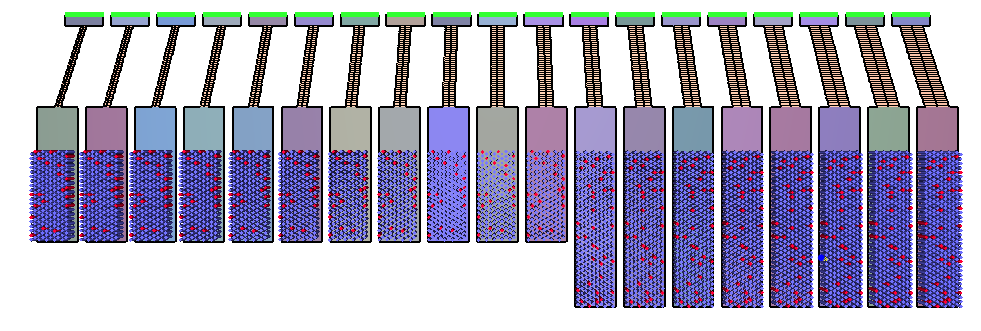
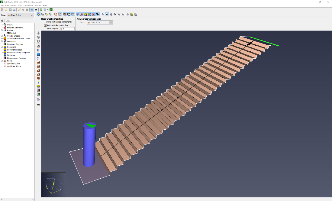
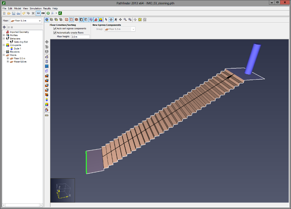
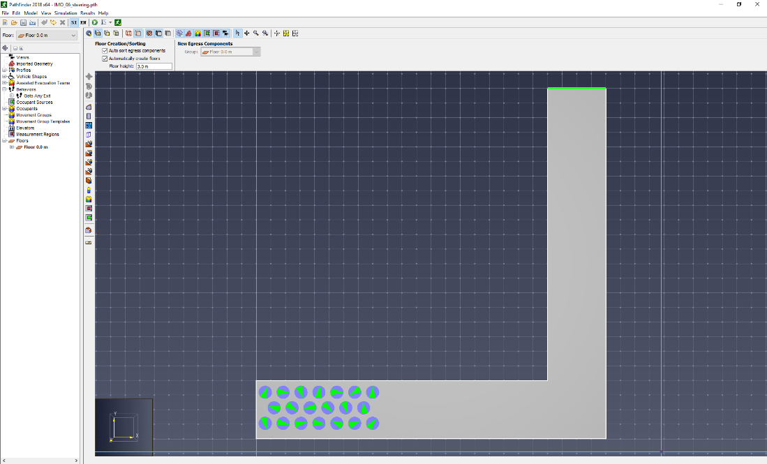
The Pathfinder model is shown in Figure 5.
This model is a subset of the experiments reported in "Transitions in pedestrian fundamental diagrams of straight corridors and T-junctions" (Zhang et al. 2011).
The Pathfinder model uses a 3 m corridor.
For six cases the entrance width varied from 2 m to 3 m with the exit width held constant at 3 m (these are low density cases) followed by 10 cases where the entrance width was held constant at 3 m and the exit width varied from 3 m to 1 m (high density cases).
The red rectangles indicate the regions used to measure the speed-density results.
To ensure steady-state results, 1000 people were used for each case.
The sixteen cases were repeated for three walking speed assumptions:
1.55 ± 0.18 m/s with the speed profile shown in Figure 6 (which represents the experimental speed-density data shown in Figure 3).1.19 m/s with the SFPE speed-density relationship (Figure 1).1.19 ± 0.25 m/s, with the with the SFPE speed-density relationship (Figure 1).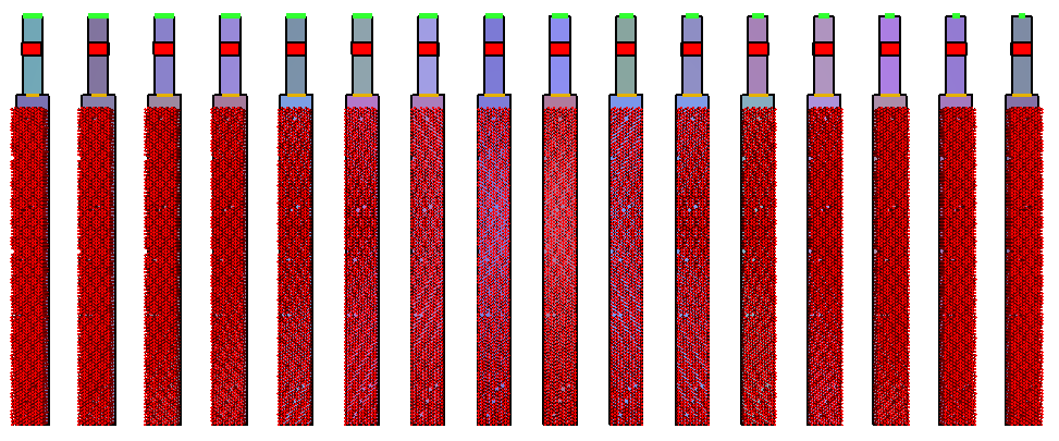

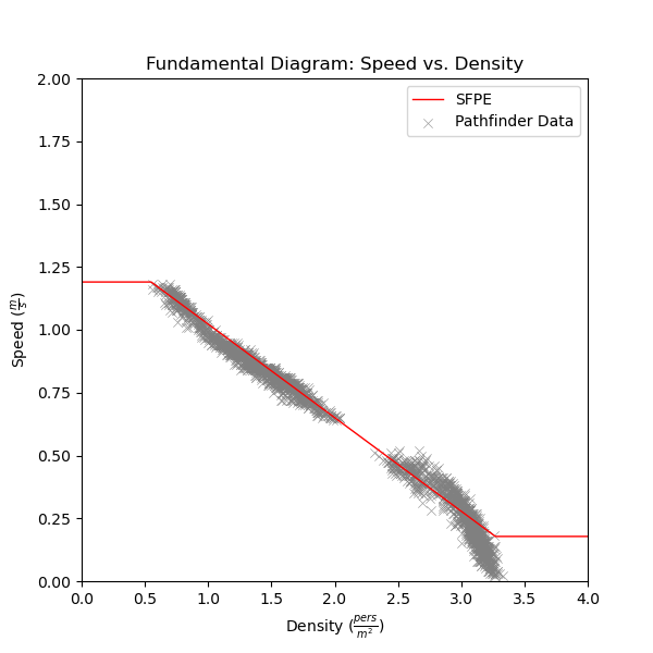
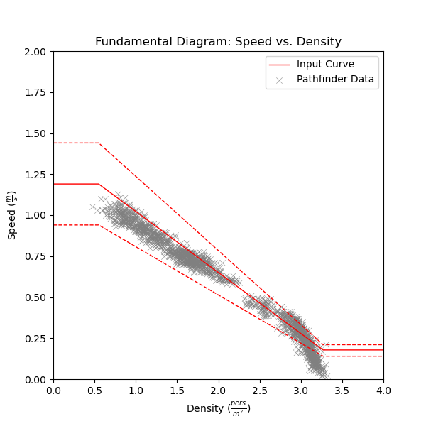
Speed-density and specific flow-density results for the Zhang and Seyfried experiment are presented for each of the three cases. In these curves, the data is presented over time intervals when "steady-state" conditions have been reached. The gray points represent all the calculated speed-density pairs for all corridors.
1.55 ± 0.18 m/s. | 1.55 ± 0.18 m/s. |
 1.19 m/s. |  1.19 m/s. |
 1.19 ± 0.25 m/s. | 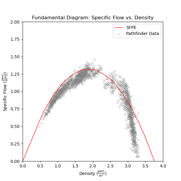 1.19 ± 0.25 m/s. |
The Pathfinder calculations replicate the input speed-density curve. The calculated points are slightly below the input curves, making the results slightly conservative. The specific flow calculations also match the expected results. The comparisons show that Pathfinder correctly uses the input speed-density curve in the calculations.
In addition to unidirectional flow, Zhang and Seyfried (Zhang and Seyfried 2013) and Zhang, Klingsch, Schadschneider, and Seyfried (Zhang et al. 2011) describe experimental results for bidirectional flow. The experimental bidirectional results are summarized and compared to unidirectional results in Figure 3.
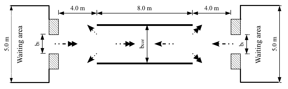
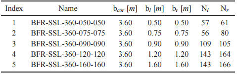
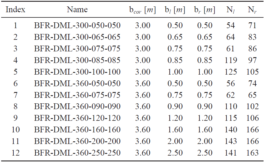
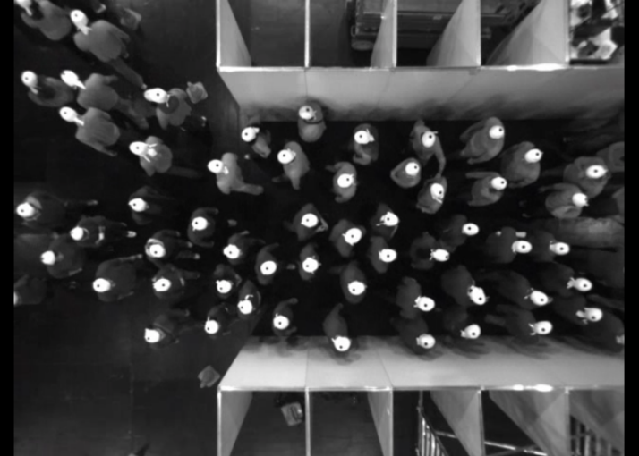
The experimental setup is shown in Figure 13. For a Balanced Flow Ratio (BFR) the left and right entrance widths were identical. A limited number of tests used an Unbalanced Flow Ratio (UFR) with different entrance widths. The measured fundamental diagrams were the same for balanced and unbalanced flow.
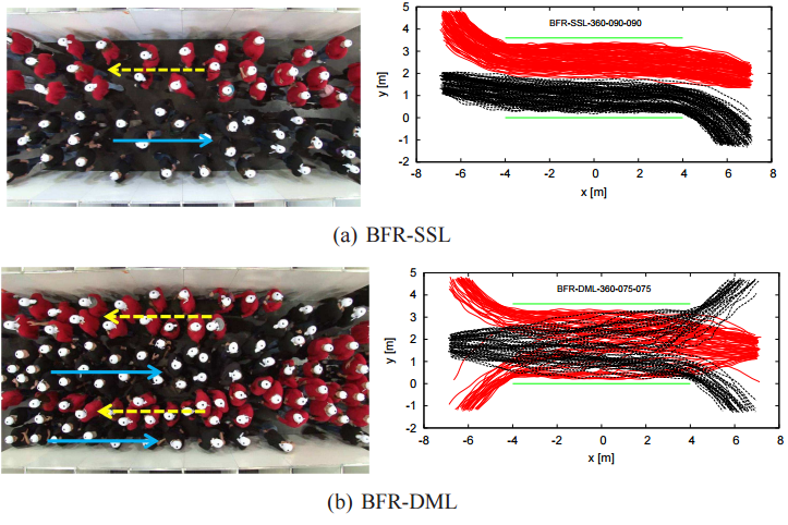
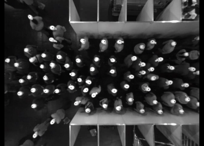
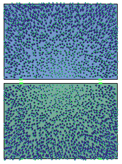
In addition, participants were either allowed to select to exit to their left or right or were assigned a direction. When the participants selected the exit direction, Stable Separated Lanes (SSL) formed, but when required to exit a given direction, lanes were unstable and varied in time and space (Figure 14) resulting in Dynamical Multi-Lanes (DML) flow.
Figure 15 and Figure 16 show the parameters for the experiments.
You can download the actual experimental videos and supporting documentation at this link, Pedestrian Dynamics Data Archive.
This validation case will focus on bidirectional flow results.
Pathfinder models were used to simulate the experimental cases with a 3.6 m wide corridor.
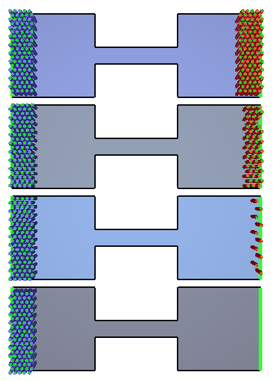
The BFR-SSL model is shown in Figure 17.
The widths of the two entry doors are always identical to each other, but the door widths change to control the density.
The red rectangles indicate the regions used to measure the speed-density results.
The measured experimental entry flow rates were used to specify the source time histories and the Enforce Flow Rate option was used.
For all cases, the measured walking speed of 1.55 ± 0.18 m/s was used with a speed profile that corresponds to the unidirectional speed-density data shown in Figure 6.
We did not modify the speed-density profile for different problems, but use the unidirectional speed-density data for all cases.
The intent is that the movement algorithm should adjust for different situations.
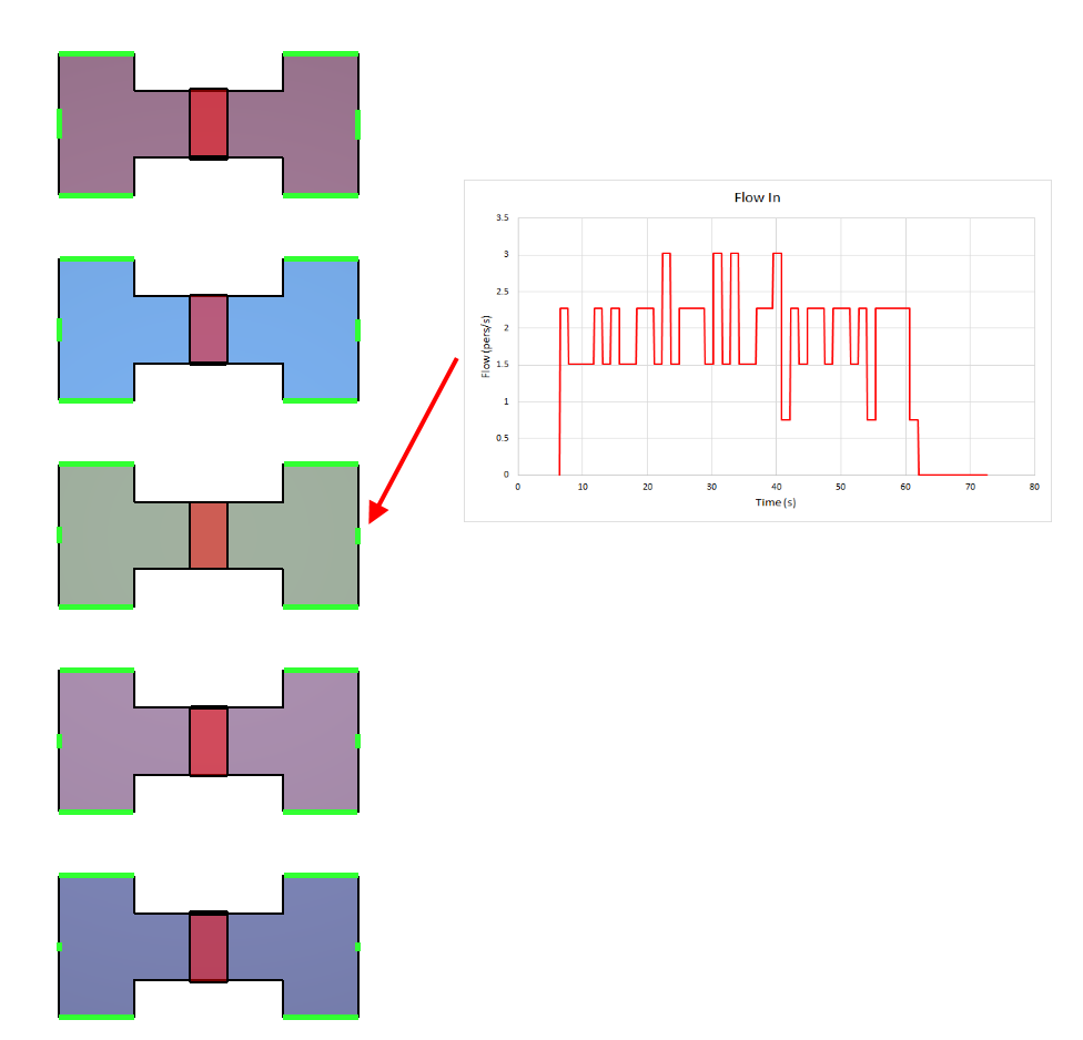
In Figure 17, the measured experimental entry flow rates are used to specify the input flows in the model. This model shows the BFR-SSL experiments, a similar model was used for the BFR-DML cases.
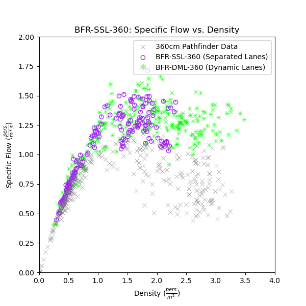
Speed-density and specific flow-density results are presented in Figure 18 and Figure 19. In these curves, the data is presented over time intervals when "steady-state" conditions have been reached. The gray points represent all the calculated speed-density pairs for all corridors.
Figure 20 and Figure 21 provide a comparison of experimentally observed and calculated occupant paths at 50 seconds, 1.6 m entry width, free choice of destination.
As shown in Figure 14 (a) and Figure 20, in the experiment occupants separated into separate lanes and maintained that separation throughout the experiment.
Occupants exited through only the corridor door on the side of their lane.
In Pathfinder, lanes form, but they are dynamic and occupants exit on both corridor doors.
 |  |
 |  |
Speed-density and specific flow-density results are presented for each of the three walking speed cases in Figure 22 and Figure 23. In these curves, the data is presented over time intervals when "steady-state" conditions have been reached. The gray points represent all the calculated speed-density pairs for all corridors, while the black points are the averaged values for each corridor.
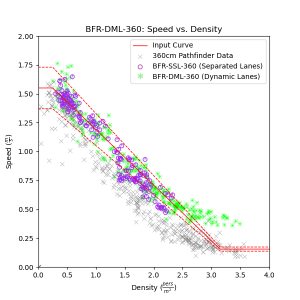 | 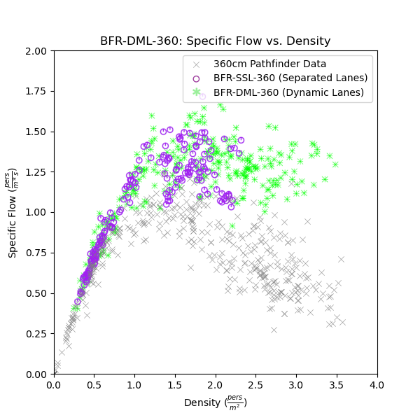 |
Figure 24 and Figure 25 provide a comparison of experimental and Pathfinder results at 30 seconds, 1.6 m entry width, assigned destination.
 |  |
Pathfinder includes only a simple lane-forming algorithm, so it does not replicate the ordered paths shown in Figure 14. Instead, the occupants tend to cross paths more frequently. As a result, for a given speed the calculated speed-density relationship and specific flow fall below the experimental data. At high densities, both can be reduced by factors of two or more.
We can explore this further by looking at the times for all occupants to pass through the corridor. Table 1 shows the corridor residence times calculated by subtracting the time the first occupant enters the corridor from the time the last occupant exits the corridor. As can be seen, at low densities the Pathfinder results are similar to experimental results. However, at high densities the Pathfinder residence times increase significantly.
This may be considered a conservative, non-optimal result.
| Case | texp | tpath | tpath/texp |
|---|---|---|---|
| BFR-SSL: Balanced Flow Ratio - Stable Separated Lanes | |||
| bo-360-050-050 | 57.0 | 70.47 | 1.24 |
| bo-360-075-075 | 67.1 | 74.75 | 1.11 |
| bo-360-090-090 | 61.7 | 110.42 | 1.79 |
| bo-360-120-120 | 78.0 | 197.53 | 2.53 |
| bo-360-160-160 | 77.2 | 180.50 | 2.34 |
| BFR-DML: Balanced Flow Ratio - Dynamical Multi-Lane | |||
| bot-360-050-050 | 66.7 | 76.95 | 1.15 |
| bot-360-075-075 | 50.5 | 64.40 | 1.28 |
| bot-360-090-090 | 63.1 | 101.20 | 1.6 |
| bot-360-120-120 | 80.0 | 171.60 | 2.15 |
| bot-360-160-160 | 76.5 | 189.07 | 2.47 |
| bot-360-200-200 | 73.9 | 183.72 | 2.49 |
| bot-360-250-250 | 72.2 | 194.85 | 2.7 |
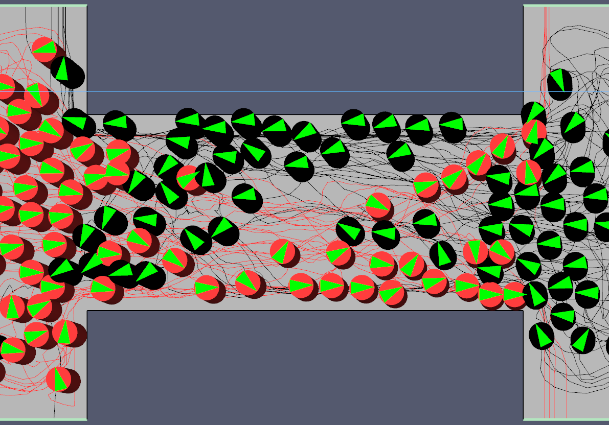
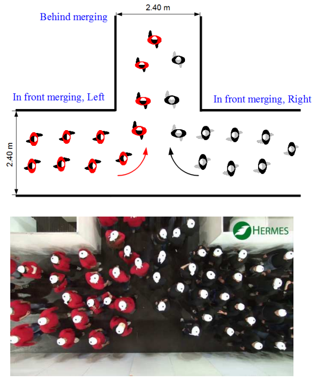
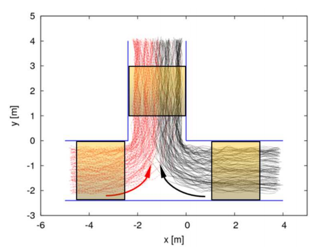
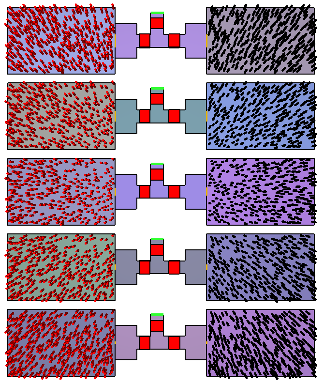
A series of experiments were performed to measure the fundamental diagram for turning and merging of pedestrian streams in T-junction (Zhang et al. 2011) (Figure 26).
The corridor width was 2.4 m and density was controlled by using different widths of the entrance (from 0.5 m to 2.4 m), which is 4 m away from the corridor.
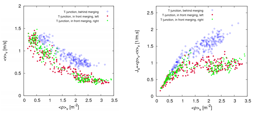
A summary of the results for unidirectional and bidirectional flows is shown in Figure 28.
The Zhang et al. experiments have an occupant speed of 1.55 ± 0.18 m/s.
As can be seen, the fundamental diagrams in front of the T-junction are different that the behind the junction.
The authors state "However, we cannot conclude whether the merging behavior itself or the congestions caused by it lead to the difference at present."
The corresponding Pathfinder model is shown in Figure 29.
The paper does not provide the exact values of entrance widths to the 2.4 m corridor, so the Pathfinder calculation assumed five cases where the entrance widths were 0.5 m, 1.0 m, 1.5 m, 2.0 m, 2.4 m.
The five cases used the Zhang and Seyfried values of 1.55 ± 0.18 m/s with a speed profile that corresponds to the speed-density data shown in Figure 3.
This input curve is shown in Figure 6.
Thus, we used the same speed-density curve for our calculations as was determined based on the independent unidirectional flow experiments.
We did not try to adjust the speed-density curve for the T-junction calculations.
This curve results in a maximum specific flow of 1.45 pers/s-m at a density of 1.736 pers/m2 and speed of 0.835 m/s.
Speed-density and specific flow-density results are presented in Figure 30 and Figure 31.
The data is presented over time intervals when "steady-state" conditions have been reached.
The calculated points for the in front measurements tend to either lie at low densities (0.0 to 0.5 pers/m2) or at higher densities (2 to 3 pers/m2).
The reason is that for the smaller entrance cases (0.5 m and 1`.0 m` width entry doors), no queues develop and so the densities stay low.
However, when the entrances are larger (1.5 m to 2.4 m), then the supply flow is larger than can be supported by the exit width, so queues form.
The queues cause the higher densities.
As previously mentioned, the specified speed-density profile was based on the unidirectional flow experiments. As can be seen, the behind data (and most of the in front data) lie on the specified curve.
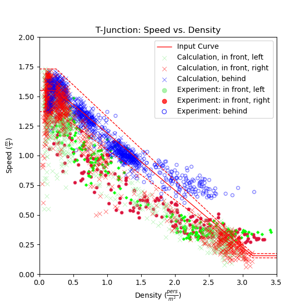 1.55 ± 0.18 m/s. | 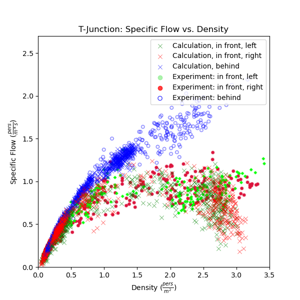 1.55 ± 0.18 m/s. |
The Pathfinder calculations replicate the input speed-density curve. For the experiments, the measured "behind" data was similar to the unidirectional experimental data. However, the "in front" data had lower speeds for a given density. The Pathfinder results show the same effect. This is likely due to merging and turning behavior as the streams merge.
In general, the Pathfinder results match the experimental data satisfactorily. It is important to remember that we used a speed-density relationship based on unidirectional data. We did not modify the curve to better match the experimental results, so Pathfinder captures the measured differences between the "behind" data and the "in front" data.
Pathfinder allows the user to define customized fundamental diagrams for movement up and down stairs and ramps. These are defined in the profiles, so now it is possible for each profile to have five fundamental diagrams (level, stairs up, stairs down, ramp up, ramp down) with different nominal speeds for each case (including the possibility of different distributions). While potentially complex, this give required flexibility to meet evacuation calculation standards required in some jurisdictions.
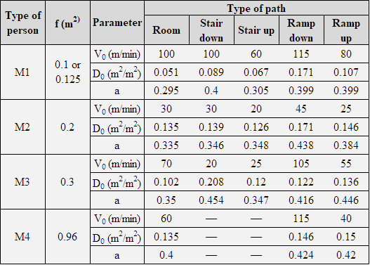
In this verification example, we will use one profile and define five different fundamental diagrams. The fundamental diagrams will correspond to the Russian evacuation code mobility profiles (M1-M4), shown in Figure 32.
In the Russian standards there are 4 types of person:
M1 - healthy person
M2 - older person or blind person or other disabled person
M3 - person with crutches
M4 - person in wheelchair
Speed depends of occupants' density:
\(D < D_{0}, V_{D} = V_{0}\)
\(D>D_{0}\), \(V_{D}=V_{0}\left(1-a\:\ln{\left(\frac{D}{D_{0}}\right)}\right)\)
Where:
\(V_{D}\) is person speed.
\(V_{0}\) is maximum velocity.
People go with \(V_{0}\) if nobody has influence on them.
D is occupant density (m2/m2) or fraction of occupied area.
\(D = \frac{Nf}{S}\)
Where:
N is number of people in area
f is area occupied by a person, m2
S is the area, m2
For the healthy population (M1), the calculated fundamental diagrams are shown in Figure 33.

Pathfinder models were used to simulate the Russian evacuation code for healthy people with a 0.1 m2 area for each person.
Five models were used, corresponding to level walking, stairs up, stairs down, ramp up, ramp down.
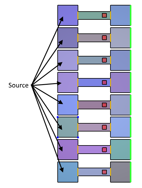
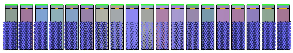
Because we are not replicating a specific set of experiments, we used room sources to supply the occupants.
The level model is shown in Figure 35, the sources are the rooms on the left and the occupants exit to the right. The sources introduce occupants to the model, the red squares indicate where speed-density is measured, and the occupants exit on the right. To control the densities, the source rate of the entry room and the flow rates of the exit doors were specified, as shown in Figure 34.
The values are different for different cases since the speed-density curves are different and different flow rates can be maintained. Similar models were used for stairs and ramps.

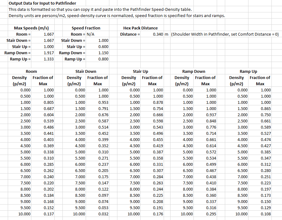
The input to Pathfinder consists of the speed (or speed ratio) for each case and the normalized speed-density curve, Figure 36.
In addition, it is necessary to set the occupant size to correspond to the person density defined by the standard.
Knowing the density, we can assume tight hexagonal packing as follows:
\(\rho_{\text{HEX}} = \frac{2}{\left( \left( \sqrt{3} \right) S^{2} \right)}\)
or:
\(S = \sqrt{\frac{2}{\left( \left( \sqrt{3} \right)\rho_{\text{HEX}} \right)}}\)
Where:
S is the spacing distance between centers of the hex-packed circles.
For a density of 10 pers/m2 the spacing is 34 cm.
In addition, it is necessary to set the corresponding comfort distance to zero.
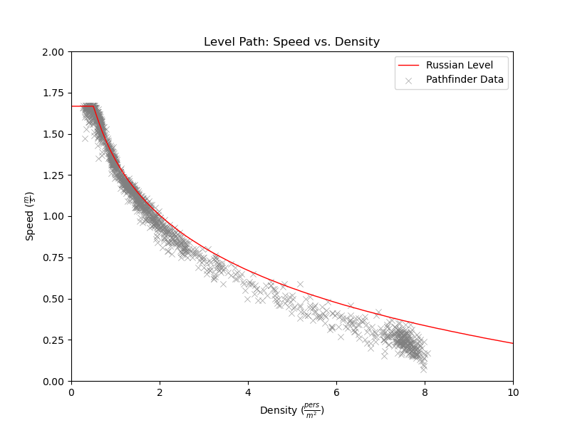
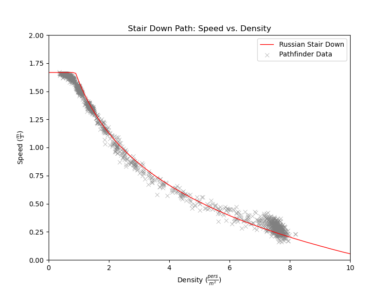
Speed-density results are presented for each of the five path types (level, stairs up, stairs down, ramp up, ramp down). In these curves, the data is presented over time intervals when "steady-state" conditions have been reached. The gray points represent all the calculated speed-density pairs for all corridors, while the black points are the averaged values for each corridor.
 |  |
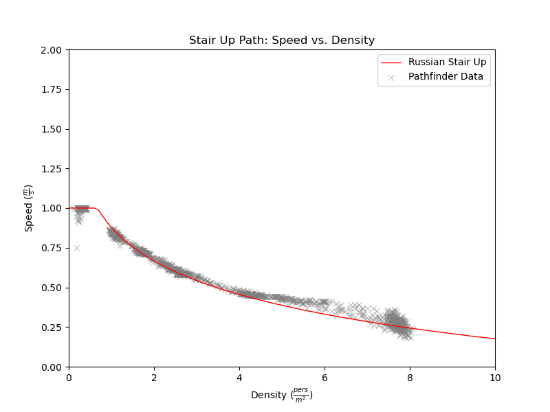 | 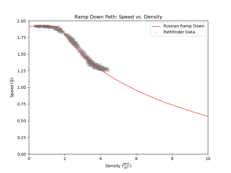 |
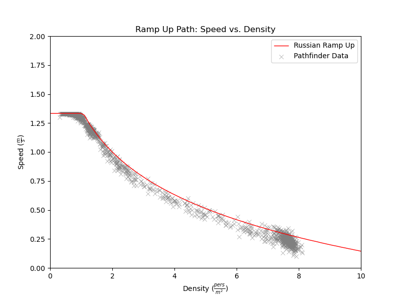
These results show that Pathfinder correctly uses the specified speed-density curves for the five different five path types (level, stairs up, stairs down, ramp up, ramp down).
For the ramp down case which has specific flows much higher than possible on level space, the Pathfinder movement algorithm limited the maximum density to about 4 pers/m2.
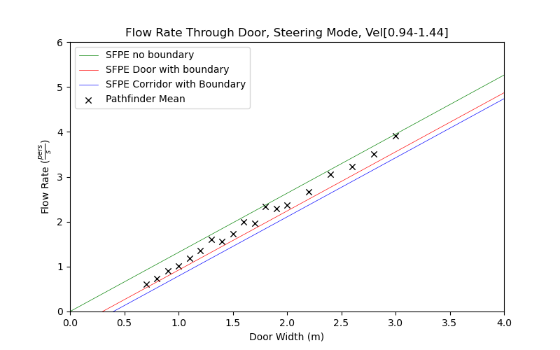
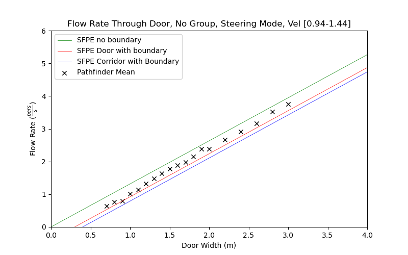
This test verifies the Pathfinder door flow rate calculation.
In steering mode, the door flow rates are not specified, but are emergent behavior based on the occupant movement.
SFPE calculates the door flow rates based on the maximum specific flow of 1.316 pers/s-m.
For doors, the specified boundary layer is 0.15 m, so a 1 m wide door is calculated to flow at 0.92 pers/s.
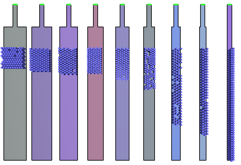
The corresponding Pathfinder model is shown in Figure 42.
The door widths range from 0.7 m to 3.0 m, with the entry corridor width 5 m.
Two Steering Mode cases were run, one with a constant velocity of 1.19 m/s and one with a uniform velocity distribution of 1.19 ± 0.25 m/s.
In addition, SFPE mode and Steering+SFPE mode cases were run for a uniform velocity distribution of 1.19 ± 0.25 m/s
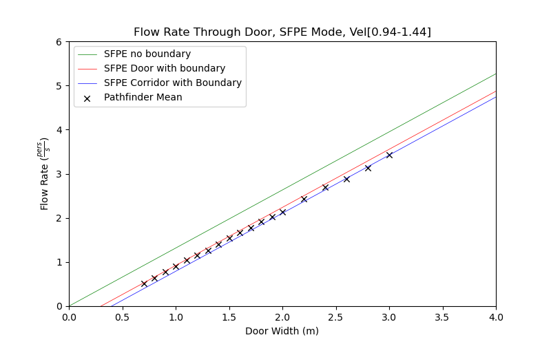
The door flow rates are shown in Figure 43 through Figure 46. This data has been averaged over the time periods where the different doors have attained "steady state" flow. For comparison, the red lines show the SFPE flow rate for the door width and a 0.15 m boundary.
 |  1.19 ± 0.25 m/s. |
 1.19 ± 0.25 m/s. | 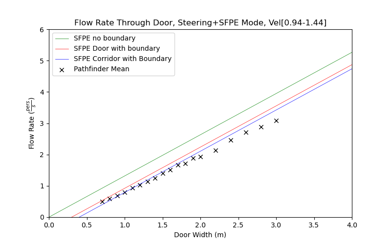 1.19 ± 0.25 m/s. |
The Pathfinder Steering mode calculations give slightly higher door flow rates than predicted using the SFPE calculations. The Pathfinder SFPE mode results are essentially identical to the SFPE predictions. The Steering+SFPE mode results are somewhat lower than the SFPE predictions.
The predictions are satisfactory.
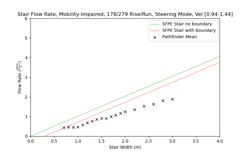
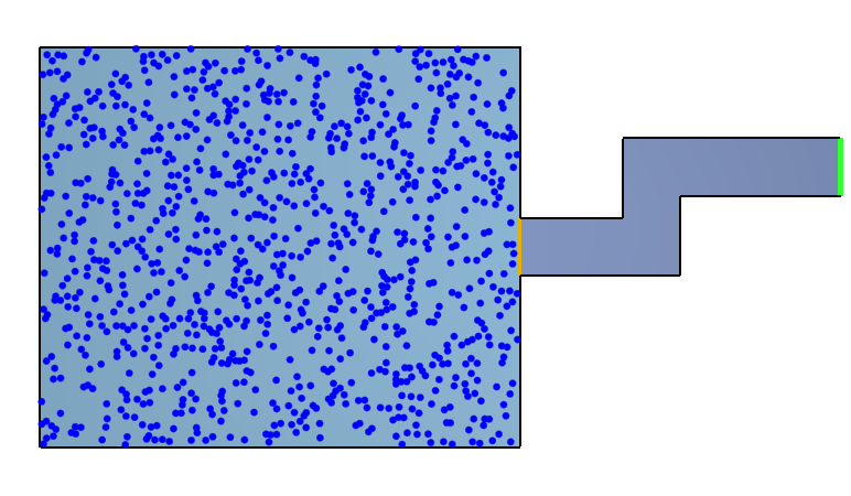
This test verifies the Pathfinder stair flow rate calculation.
In steering mode, the stair flow rates are not specified, but are emergent behavior based on the occupant movement, including maximum speed as a function of stair riser/tread dimensions and occupant density.
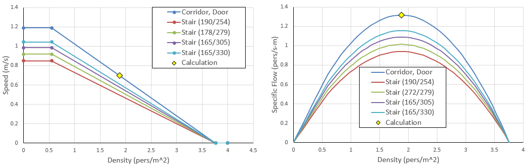
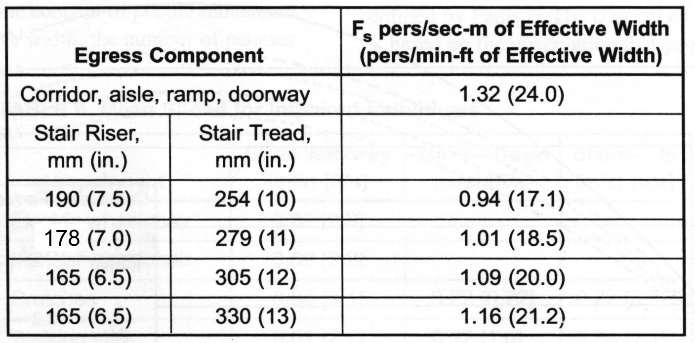
SFPE calculates the stair flow rates based on the maximum specific flow that is a function of riser/tread dimensions, see Figure 47.
For stairs, the specified boundary layer is 0.15 m, so a 1 m wide stair with rise/run of 178/279 is calculated to flow at 0.71 pers/s.
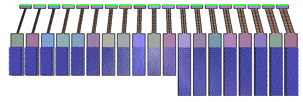
The corresponding Pathfinder model is shown in Figure 48.
The door widths range from 0.7 m to 3.0 m. Entry corridor width is 5 m. Stairs have a total rise of 7 m and a run of 11 m.
Two Steering Mode cases were run, one with a constant velocity of 1.19 m/s and one with a uniform velocity distribution of 1.19 ± 0.25 m/s.
In addition, SFPE mode and Steering+SFPE mode cases were run for a uniform velocity distribution of 1.19 ± 0.25 m/s
The stair flow rates are shown in Figure 49 through Figure 52.
This data has been averaged over the time periods where the different stairs have attained "steady state" flow.
For comparison, the red lines show the SFPE flow rate for the stair width and a 0.15 m boundary.
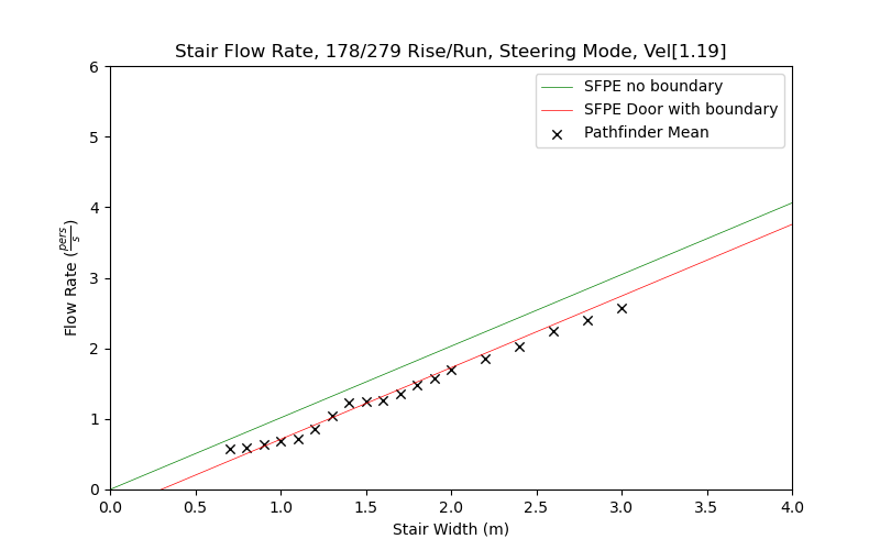 1.19 m/s. |  1.19 ± 0.25 m/s. |
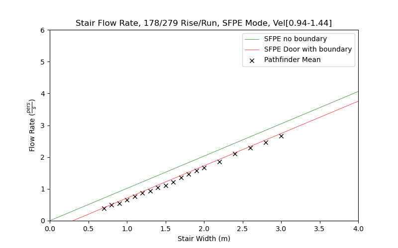 1.19 ± 0.25 m/s. |  1.19 ± 0.25 m/s. |
The Pathfinder Steering mode calculations lie close to the SFPE calculations. The Pathfinder SFPE mode results are essentially identical to the SFPE predictions. The Steering+SFPE mode results are somewhat lower than the SFPE predictions.
The predictions are satisfactory.
This test is similar to the door flow rate verification but examines flow rates through corridors for which SFPE species a 0.2 m boundary layer (a 1 m corridor has a 0.79 pers/s flow rate).
It also tests the sensitivity of Pathfinder to the width of the entry shoulder on each side of the corridor.
The Pathfinder models are shown in Figure 53 and Figure 54.
The corridor widths are 1 m and 3 m and the shoulder widths range from 0 to 2 m.
Steering Mode cases were run, one with a constant velocity of 1.19 m/s and one with a uniform velocity distribution of 1.19 ± 0.25 m/s.
In addition, SFPE mode and Steering+SFPE mode cases were run for a uniform velocity distribution of 1.19 ± 0.25 m/s
1 m wide corridor flow rates.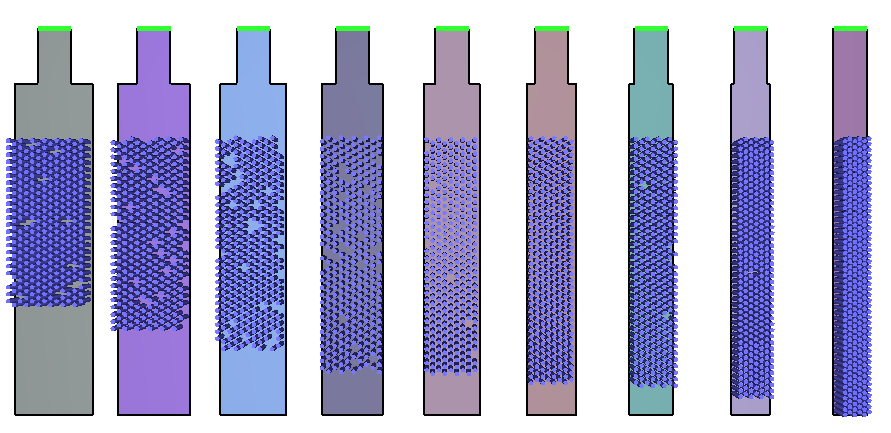
3 m wide corridor flow rates.The corridor flow rates are shown in Figure 55 through Figure 62. This data has been averaged over the time periods where the different doors have attained "steady state" flow. For comparison, the blue lines show the SFPE corridor flow rate.
 1 m corridor in Steering Mode with varying entry shoulder widths. Occupants have a constant max speed of 1.19 m/s. | 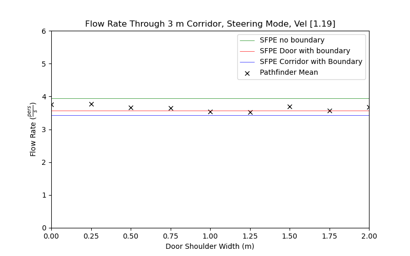 3 m corridor in Steering Mode with varying entry shoulder widths. Occupants have a constant max speed of 1.19 m/s. |
 1 m corridor in Steering Mode with varying entry shoulder widths. Occupants have a max speed distribution of 1.19 ± 0.25 m/s. | 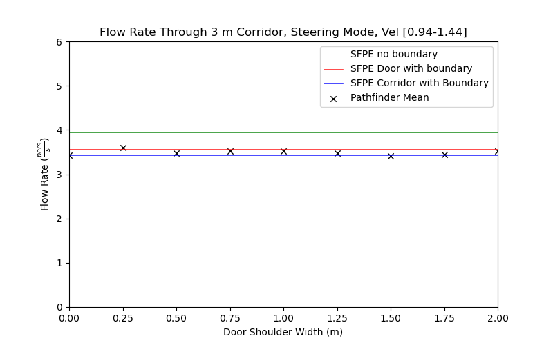 3 m corridor in Steering Mode with varying entry shoulder widths. Occupants have a max speed distribution of 1.19 ± 0.25 m/s. |
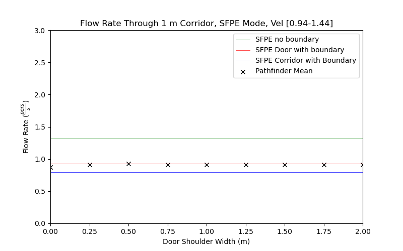 1 m corridor in SFPE Mode with varying entry shoulder widths. Occupants have a max speed distribution of 1.19 ± 0.25 m/s. |  3 m corridor in SFPE Mode with varying entry shoulder widths. Occupants have a max speed distribution of 1.19 ± 0.25 m/s. |
 1 m corridor in Steering+SFPE Mode with varying entry shoulder widths. Occupants have a max speed distribution of 1.19 ± 0.25 m/s. | 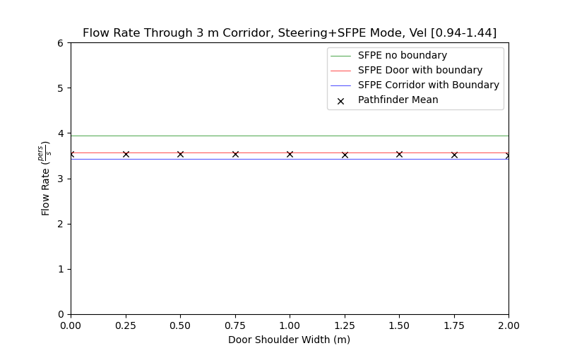 3 m corridor in Steering+SFPE Mode with varying entry shoulder widths. Occupants have a max speed distribution of 1.19 ± 0.25 m/s. |
For the 1 m wide corridor, the Pathfinder calculations give slightly higher flow rates than predicted using the SFPE calculations.
For the 3 m door, the flow rates are nearly identical to the SFPE calculations.
The results are not sensitive to the width of the entry shoulder.
For SFPE mode, the corridor width does not affect the calculation, so the flow rates are controlled primarily by the exit door flow rate. Also for SFPE mode, when the corridor is the same width as the entry room, the density in the corridor/entry room slows the walking speed so the zero shoulder width corridor cases show slightly lower flow rates.
The correlation between the Pathfinder calculations and the expected flow rates is satisfactory.
This tests simple behaviors, including exits and a refuge room.
150 occupants were evenly divided with three different behaviors: go to one of two exits or go to the refuge room (a final destination).
The occupants were initially located in one room and then proceed to their exits as shown in Figure 63.
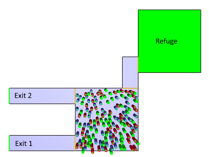
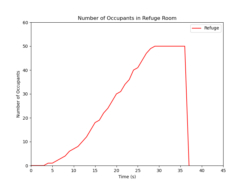
Figure 64 shows a plot of the refuge room usage.
The 50 occupants assigned to use the refuge did so.
The same results were obtained for SFPE and Steering+SFPE modes.
The occupants proceeded to use the exits and refuge associated with their behaviors.
The Pathfinder calculations performed as expected.
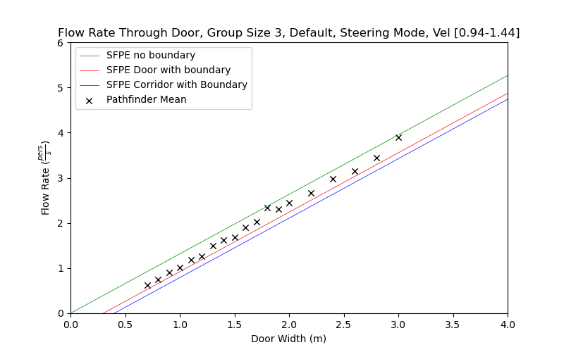
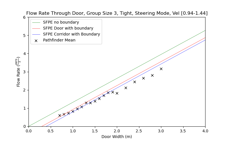
This case tests the effect of grouping on door flow rates.
We use the same model as used for the door flow rate tests, but the occupants are grouped into groups of 3 and 5 people.
The model is shown in Figure 65.
It is the same as the previous door flow rate model (steering mode with a uniform velocity distribution of 1.19 ± 0.25 m/s), except the space downstream of the doors is extended to allow group leaders to pause and wait for the rest of their group to catch up.
Dynamic grouping was used with the Number of Members in the group defined as 3 and 5 and the group minimum size of 1.
Two group formations were used: a tight group formation with a Maximum Distance of 1.0 m and a Slowdown Time of 3 s, and the default group with properties with a Maximum Distance of 2.0 m and a Slowdown Time of 3 s.
The maximum speed was defined as a uniform distribution of 1.19 ± 0.25 m/s.
As a result, members of a group will have different speeds, so the faster members slow down to keep the group together.

Figure 66 through Figure 70 show plots of door flow rates in steering mode.
Without grouping (Figure 66) the door flow rate for the 3 m door is slightly less than the previous model.
This is due to the downstream effect of movement in the corridor that slightly slows movement through the door.
When grouped, the steering mode door flow rates do not change significantly for the default grouping parameters, but do decrease for the tight grouping parameters. This is because the tight grouping means increased delays as the group waits to reform.
Grouping in SFPE mode does not change the door flow rates, Figure 71.
Figure 72 shows the results for Steering+SFPE mode for the tight grouping with a group size of 5. These results show that the door flow rate constraint slows the door flow rate further.
 |  3. |
 3. |  5. |
 5. | 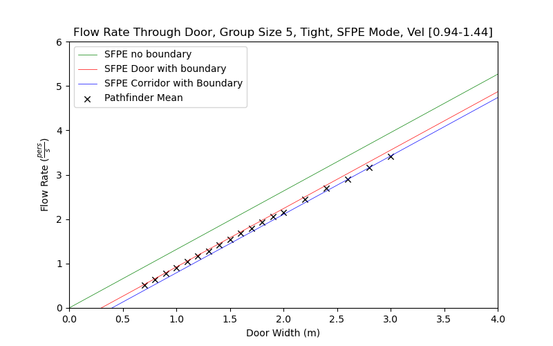 5. |
Tight groups show slower movement through doors. For the default group parameters, which allows the members of the group to become more separated, the effect on door flow rates is small.
The Pathfinder calculations performed as expected.
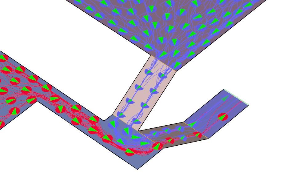
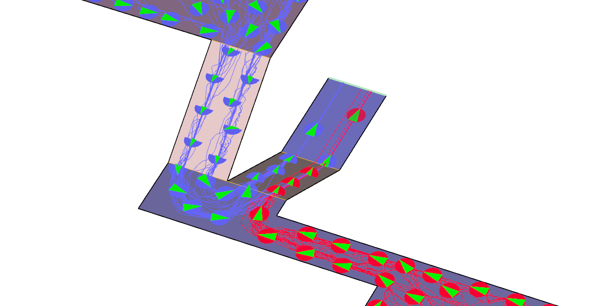
This test expands a corridor merging problem discussed by Galea et al. (Galea, Sharp, and Lawrence 2008). The problem consists of two flow streams meeting at a junction and continuing to the exit. We add a variation in corridor width to the original Galea problem. We also add a T-junction geometry as described by Zhang et al. (Zhang et al. 2011).
Figure 73 shows the Galea ("adjacent") geometry and typical merging behavior for a 3 m wide corridor. Figure 74 shows the T-junction ("opposite") geometry model with typical merging behavior. For both geometries we also solve for 1 m wide corridors.
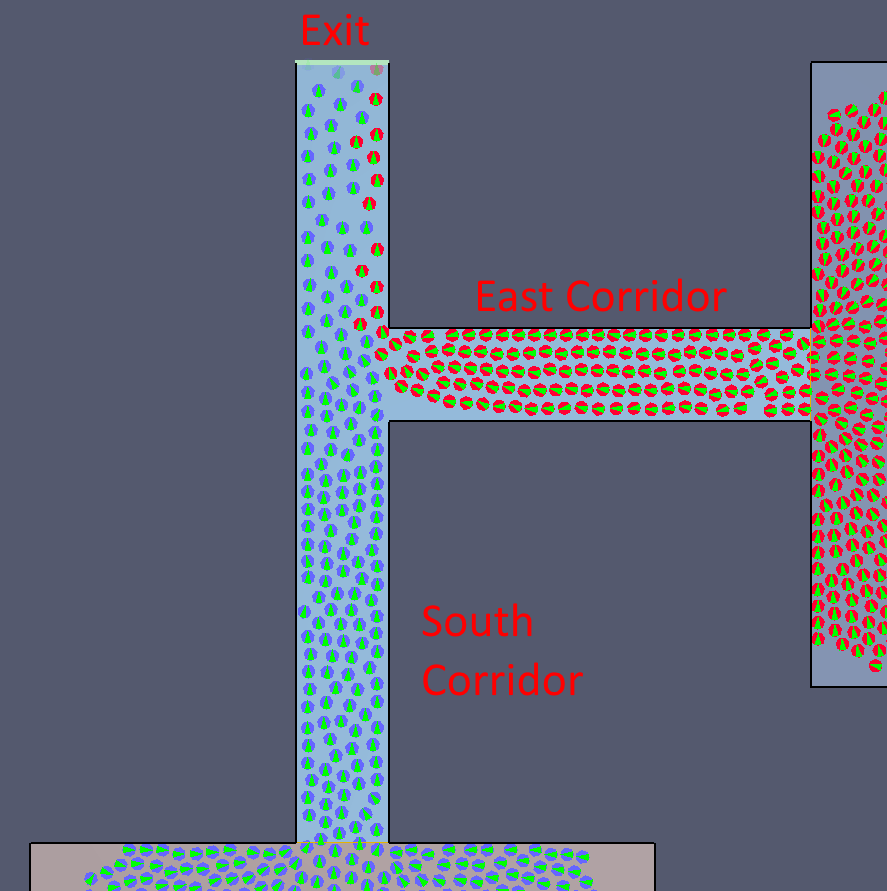
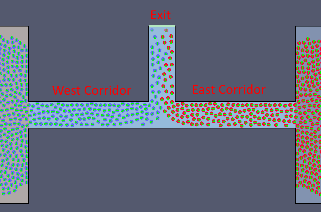
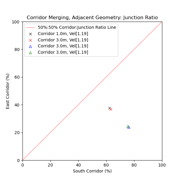
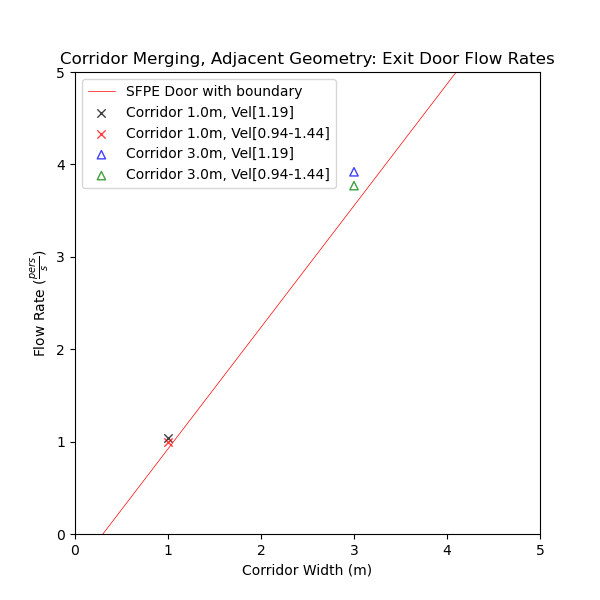
The merging ratios and exit flow rates for the adjacent geometry are shown in Figure 75 and Figure 76. These were calculated after the door flow rates had reached "steady state" values. Figure 77 and Figure 78 show the same results for the "opposite" geometry.
 |  |
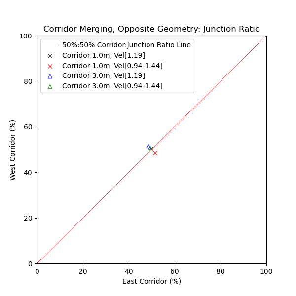 |  |
In all cases for the "opposite" geometry, the merging flows are balanced with 50:50 ratios.
This matches the Zhang et al. (Zhang et al. 2011) experimental results.
The "adjacent" geometry case is more interesting.
For a 1 m corridor, the merging ratios favor the south (straight) corridor flow (approximately 60:40).
However, for the wider 3 m corridor, the south (straight) corridor flow strongly dominates the merging behavior (approximately 75:25).
The Galea et al. (Galea, Sharp, and Lawrence 2008) paper examines the effects of different occupant "drives" on merging, but does not examine the effect of different corridor geometry.
The Pathfinder results are satisfactory.
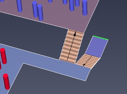
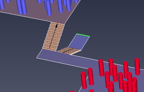
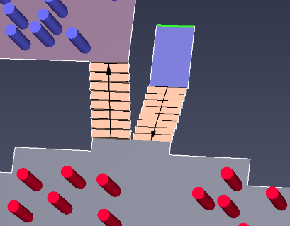
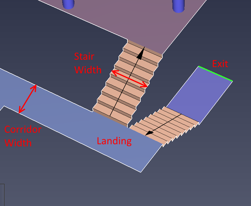
This test expands the stair merging problem discussed by Galea et al. (Galea, Sharp, and Lawrence 2008). The paper categorizes two stair merging geometries: "adjacent" (Figure 79) and "opposite" (Figure 79) defined by how the floor occupants merge at the landing relative to the occupants descending the stairs. We have added a third "open" geometry in which the floor has direct access to the exit stair (Figure 81).
The following images show the categorization of stair merging geometries. The arrows indicate the "up" direction on the stairs, not the flow direction.
 |  |  |
The width of the stairs was 1.5 m and solutions were made for corridor widths of 1.0 m and 1.45 m (Figure 82).
The first floor is at Z = 1.6 m and the second at Z = 3.2 m. The rise/run of the stairs is approximately 7/11 with a total stair length of 2.97 m.
For this stair, the SFPE guidelines give a speed that is 77% of the free walking speed.
Typical results for the merging behavior for the adjacent geometry with corridor widths of 1.0 m (Figure 83) and 1.45 m (Figure 84) are shown below.
For the default occupant dimensions, the 1.0 m narrow corridor requires a "staggered" walking pattern while the wider corridor enables "side by side" walking.
As a result, the floor flow is more dominant for the wider entry corridor.
The merging ratios and exit flow rates for all cases are shown in Figure 87, Figure 88, Figure 89, and Figure 90. In the "open" geometry, the floor flow dominates the merging behavior.
 1.0 m wide adjacent corridor entry | 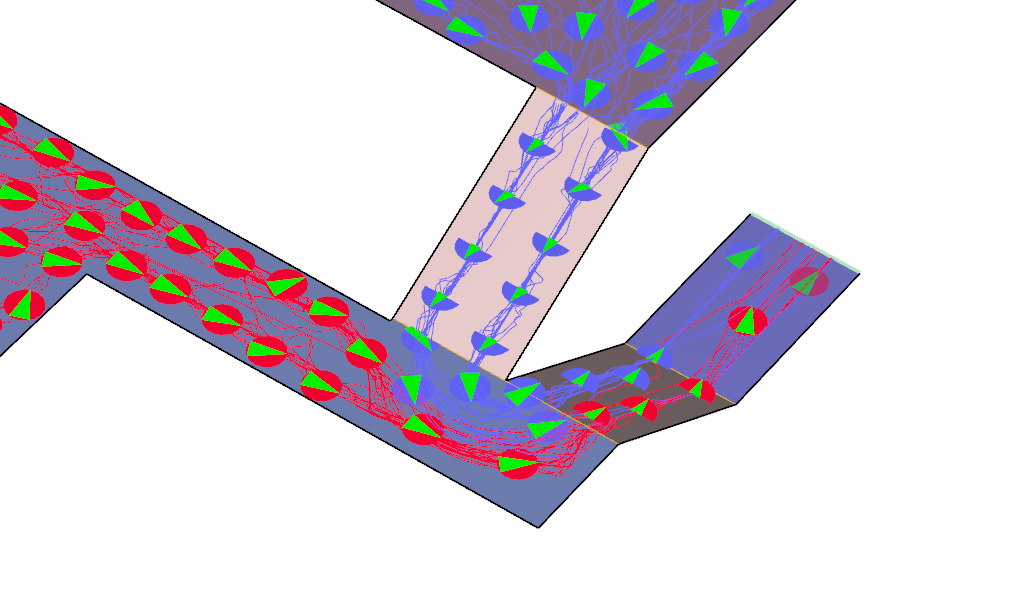 1.45 m wide adjacent corridor entry |
Typical merging behavior for the "opposite" configuration with 1.19 m/s occupant speed and different corridor entry widths are shown below.
 1.0 m wide opposite corridor entry | 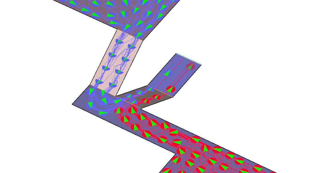 1.45 m wide opposite corridor entry |
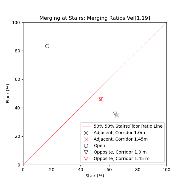 1.19 m/s. | 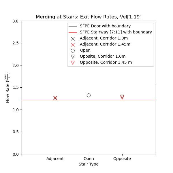 1.19 m/s. |
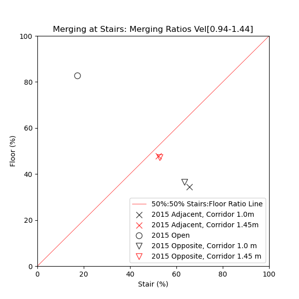 1.19 ± 0.25 m/s. |  1.19 ± 0.25 m/s. |
The calculated merging ratios fall within the range of experimental data summarized by Galea et al. (Galea, Sharp, and Lawrence 2008). The results match a general trend discussed by Galea et al. for the "opposite" geometry to favor floor merging over the "adjacent" geometry. This would appear to be related to congestion that forms at the landing. For the "adjacent" geometry both streams must merge and then proceed to the landing leading to the exit. For the "opposite" case the two streams approach the exit stair in an approximately symmetric pattern, similar to the T-junction case for corridor merging discussed above.
However, it should be noted that Boyce et al. states, "The results indicate that, despite differences in the geometrical location of the door in relation to the stair and the relative stair/door width, the merging was approximately 50:50 across the duration of the merge period in each of the buildings studied." (Boyce, Purser, and Shields 2012)
Their experiments noted how individual behavior could change the merge ratios.
The exit flow rates are controlled by the stair flow rate, not the exit door capacity.
The Pathfinder results are satisfactory.
This test evaluates the Pathfinder capability to simulate passing behavior around slow occupants on stairs. For this behavior, it is expected that when the stair width is sufficient, faster occupants will pass slower occupants on stairs.
However, the actual effect of disabled or wounded occupants on stairs can be complex. Averill et al. in their report on occupant behavior and egress in the World Trade Center disaster (Averill et al. 2005) noted the following different situations:
In modeling, the user must be aware of these situations and model accordingly.
The same model used for the stair width study was used for this study.
The door widths range from 0.7 m to 3.0 m, with the entry corridor width 5 m.
Stairs have a total rise of 7 m and a run of 11 m.
Two occupant profiles were defined: a default profile with a uniform velocity distribution of 1.19 ± 0.25 m/s, and a slow profile with a constant velocity of 0.5 m/s.
The 0.5 m/s velocity as a low end of the walking speeds for impaired individuals described in Figure 47 of the SFPE Handbook (SFPE 2016).
10 percent of the occupants were given the slow profile (red occupants in Figure 91).
Steering mode was used, since this is the mode in which passing behavior is used.
The stair flow rates with mobility-impaired occupants are shown in Figure 92.
This data has been averaged over the time periods where the different stairs have attained "steady state" flow.
For comparison, the red lines show the SFPE flow rate for the stair width and a 0.15 m boundary.
1.19 ± 0.25 m/s, 10 percent have a constant speed of 0.5 m/s.The presence of mobility-impaired occupants reduces the stair flow rates (compare with Figure 50). No experimental data is available for comparison, but the trend is reasonable.
This problem tests elevator loading.
100 occupants are located in a 10x10 m room at an elevation of 10 m.
The occupants exit using an elevator with dimensions 2 m wide and 1.7 m deep, for a typical elevator loading of about 16 people (Klote and Alvord 1992) and the elevator door width is 1.2 m.
The elevators have an Open+Close Time of 7.0 s, Pickup and Discharge times of 10.0 s, and Open and Close delays of 5.0 s (see the Pathfinder User Manual for more information).
There are four elevators, with specified Nominal Loads of 5, 10, 20, and 50 persons (Figure 93).
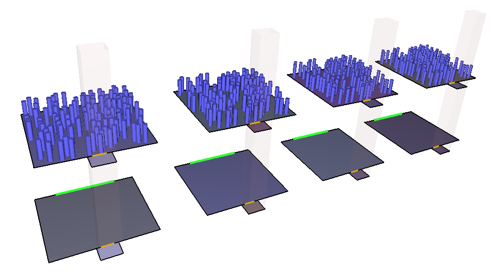
The four problems are independent, so allow a quick verification.
The resulting elevator loads for the steering simulation are shown in Figure 94 and match the expected results. The results for Steering+SFPE and SFPE modes also matched the expected results.
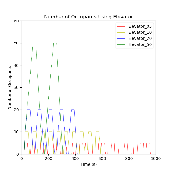
The elevator loadings matched the expected values.
This example tests the use of the corridor width while cornering.
The example was originally presented in the FDS+Evac Technical Reference and User’s Guide (Korhonen 2018).
The problem describes an assembly space filled with 1000 occupants.
The initial room measures 50 m x 60 m.
At the right, there is a 7.2 m doorway leading to a 7.2 m corridor.
The corridor contains a sharp turn to the left before continuing to the exit.
The feature of interest in this problem is the corner in the corridor. Based on how different simulators handle the flow of large groups around a corner, different simulators can produce substantially different answers. Notably, the current body of movement research presents us with little guidance toward a "correct" solution to this problem.
In addition to the two-corner problem, we simulated a single corner and a straight corridor without a corner. Only steering mode results are presented, since that is the case for which the corner slows movement.
The primary interest is in how effectively the simulator uses the full width of the corridor and corner, Figure 96. In the Pathfinder simulation, there is some grouping that occurs in the vertical section of the corridor. This is a result of increased density which leads to slower movement.
The time for all occupants to exit was 164 seconds for the straight corridor, 163 seconds for one corner, and 185 seconds with two corners.
The model with a straight corridor has a 7.2 m wide corridor and a path length from the room to the exit of 41.5 m.
An SFPE calculation using the flow rate and walking speeds at a density of 1.88 pers/m2 and gives a total time of 171 seconds.

The Pathfinder results are reasonable.
This test verifies that during assisted evacuation, the speed of the person being assisted controls the movement speed.
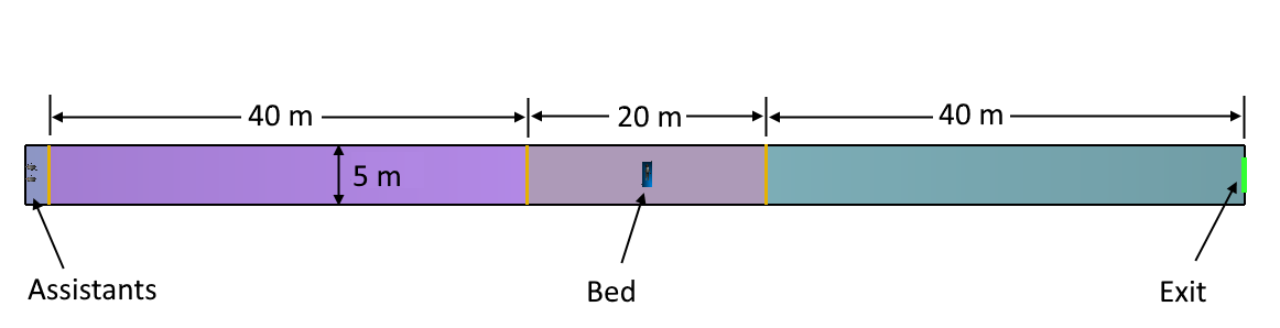
The problem consists of a corridor, with the assistants at one end and the patient needing assistance located at the center of the corridor. The assistants first move independently to the patient, then they assist the patient to the exit. Initially, the assistants will use their independent walking speeds, but when assisting will use the patient speed.
Figure 97 shows the test geometry.
The default speed of the assistants is 1.19 m/s and the speed of the bed is 1 m/s.
The speed of the assistants moving independently and assisting the bed occupant are shown in Table 2. This data was taken from the occupant csv output file.
| Mode | Speed Independent (m/s) | Speed Assisting (m/s) |
|---|---|---|
| Steering | 1.19 | 1.0 |
| SFPE | 1.19 | 1.0 |
| Steering+SFPE | 1.19 | 1.0 |
All cases correctly show the specified independent walking speed and that the speed changes to the bed speed when assisting the bed occupant.
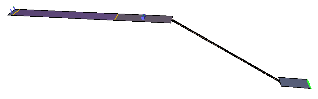
This test verifies that during assisted evacuation, the speed of the person being assisted controls the movement speed up stairs.
This test is similar to the level surface test, except the occupants now move up stairs that have a rise of 17.5 cm and a run of 29.0 cm.
The width of the stairs was 1.1 m.
The total horizontal distance of the stairs is 40 m and the vertical distance is 24 m, so the diagonal distance on the stairs is 46.64 m.
The patient speed up the stairs was specified as 0.3 m/s.

The speed of the assistants moving independently and assisting the bed occupant up the stairs are shown in the following table. This data was taken from the occupant csv output file.
| Mode | Speed Independent (m/s) | Speed Assisting (m/s) |
|---|---|---|
| Steering | 1.19 | 0.3 |
| SFPE | 1.19 | 0.79 |
| Steering+SFPE | 1.19 | 0.3 |
All cases correctly show the specified independent walking speed. For SFPE mode, the speed up the stair is defined by the SFPE correlation and not the user input.
This test verifies that during assisted evacuation, the speed of the person being assisted controls the movement speed down stairs.
This test is similar to the level surface test, except the occupants now move down stairs that have a rise of 17.5 cm and a run of 29.0 cm.
The width of the stairs was 1.1 m.
The total horizontal distance of the stairs is 40 m and the vertical distance is 24 m, so the diagonal distance on the stairs is 46.64 m.
The speed down the stairs was specified as 0.5 m/s.
The speed of the assistants moving independently and assisting the bed occupant down the stairs are shown in the following table. This data was taken from the occupant csv output file.
| Mode | Speed Independent (m/s) | Speed Assisting (m/s) |
|---|---|---|
| Steering | 1.19 | 0.5 |
| SFPE | 1.19 | 0.79 |
| Steering+SFPE | 1.19 | 0.5 |
All cases correctly show the specified independent walking speed. For SFPE mode, the speed down the stair is defined by the SFPE correction and not the user input.
This test verifies the capability to assign assistants to teams and then assign occupants that need evacuation assistance to be assisted by specific teams.
There are seven assistants: five assigned to the red team and two to the blue. The occupants that need assistance are divided equally, so that six will be assisted by the red team and six by the blue.
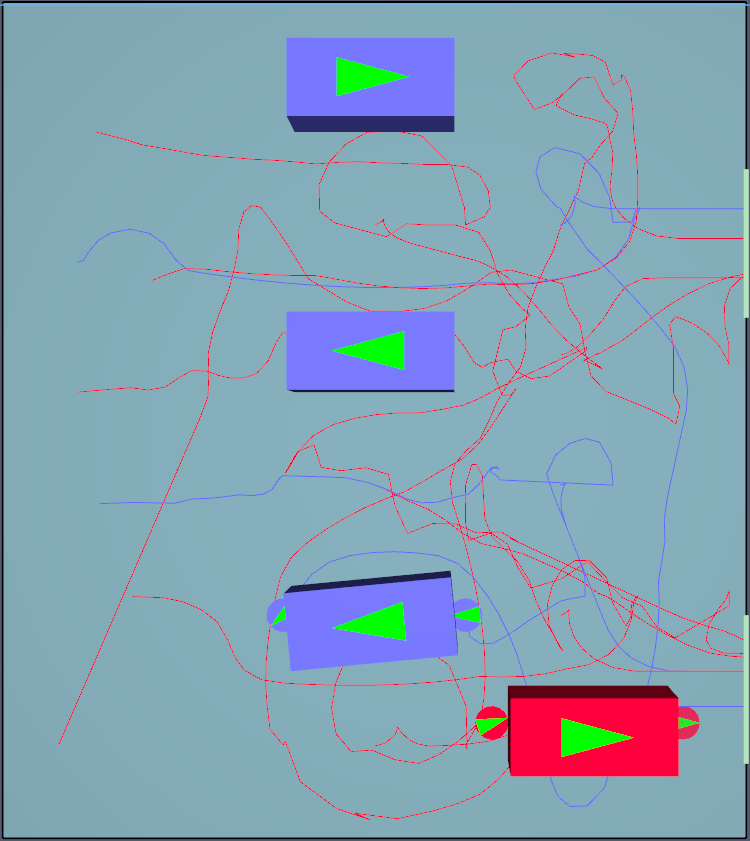
Figure 100 shows the model used to test the assignment of assist teams. The smaller occupants needing assistance are wheelchairs and the larger are beds. Each team is assigned to evacuate the wheelchairs first, then the beds.
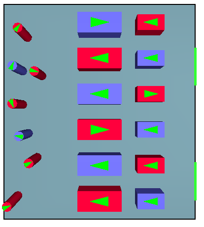
Figure 101 shows the result early in the evacuation, the wheelchairs are being assisted first. Three members of the red team are assisting wheelchairs, so the other two red team members are assisting the bed. The two blue team members are assisting wheelchairs. For assisted occupants, if a path is blocked, the assisted beds (or other vehicle) are briefly represented as cylinders to allow some overlap with the blocking wheelchairs (vehicles).
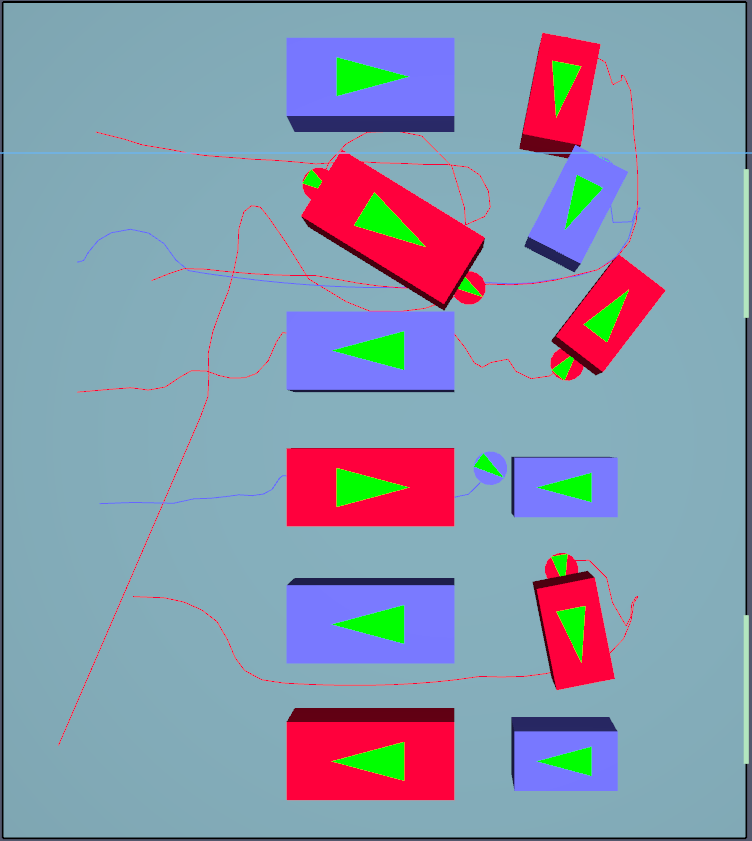
10 seconds. Note that the order of evacuation was wheelchairs first.Figure 102 shows the movement near the end of the simulation. Notice that the red occupants needing assistance have been nearly all helped. It takes longer to assist the blue occupants, since there are only two members in the blue team.
Assistants in the red team evacuated only red occupants and the blue team evacuated only blue occupants. Assisting the blue occupants took longer, since there were fewer members in the blue team.
The beds and wheelchairs moved as expected, avoiding other beds and wheelchairs when possible and, if blocked, briefly allowing some overlap.
When each team completed the assigned tasks, they exited.
The assistance behavior is as expected.
This test replicates a simulation of evacuation from the 11th floor of a hospital, as described in a paper by Hunt, et al. (Hunt, Galea, and Lawrence 2013).
As described in the paper, "Data were collected from 32 trials in which a test subject was evacuated through 11 floors of Ghent University Hospital using four commonly used movement assistance devices: stretcher, carry chair, evacuation chair and rescue sheet."
Using this data, simulations of the evacuation of 28 patients were made using different devices, different numbers of staff, and male/female teams.
We will replicate two scenarios:
Figure 103 shows the basic geometry of the hospital floor to be evacuated. In this figure, some of the dimensions such as corridor door widths have been estimated by scaling the drawing.
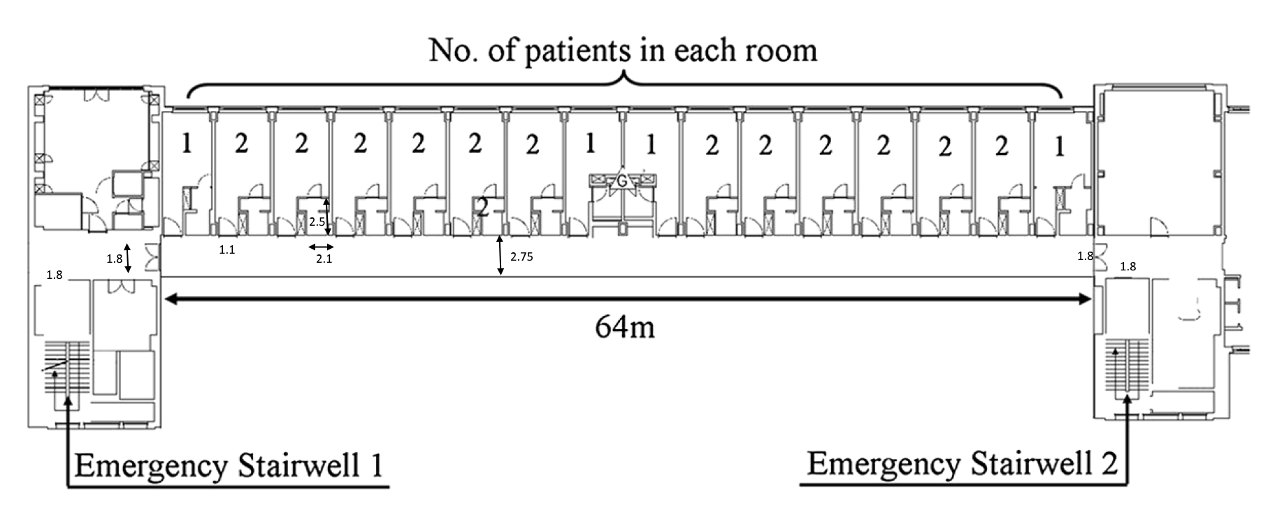
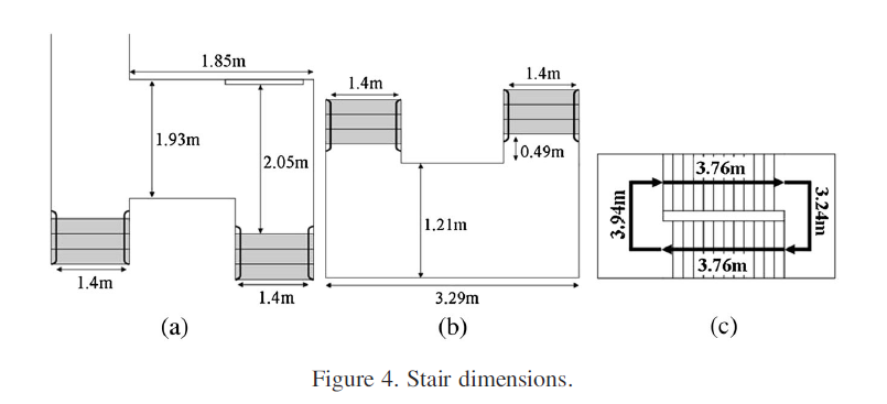
Figure 104 shows the geometry of the stairs.
Key dimensions of the stairs are that each step has a rise of 17.5 cm and a run of 29 cm, there are 12 rises in each flight of stairs (this model neglected the detail that flights between floors 2 and 3 have only 10 risers), and the width of the stairs are 1.4 m between the handrails.
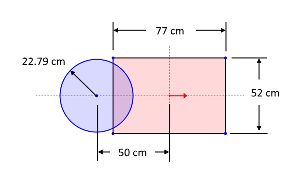
The geometry of the evacuation chair (Figure 105), evacuation stretcher (Figure 106), and assistant positions are shown below.
 1 assistant. | 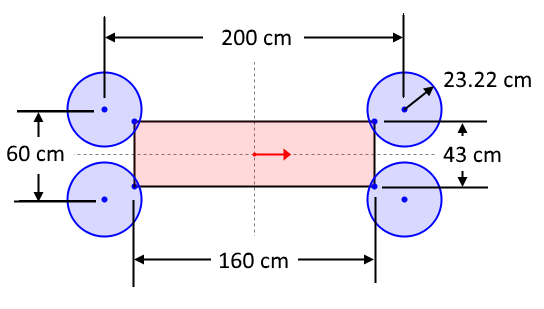 4 assistants. |
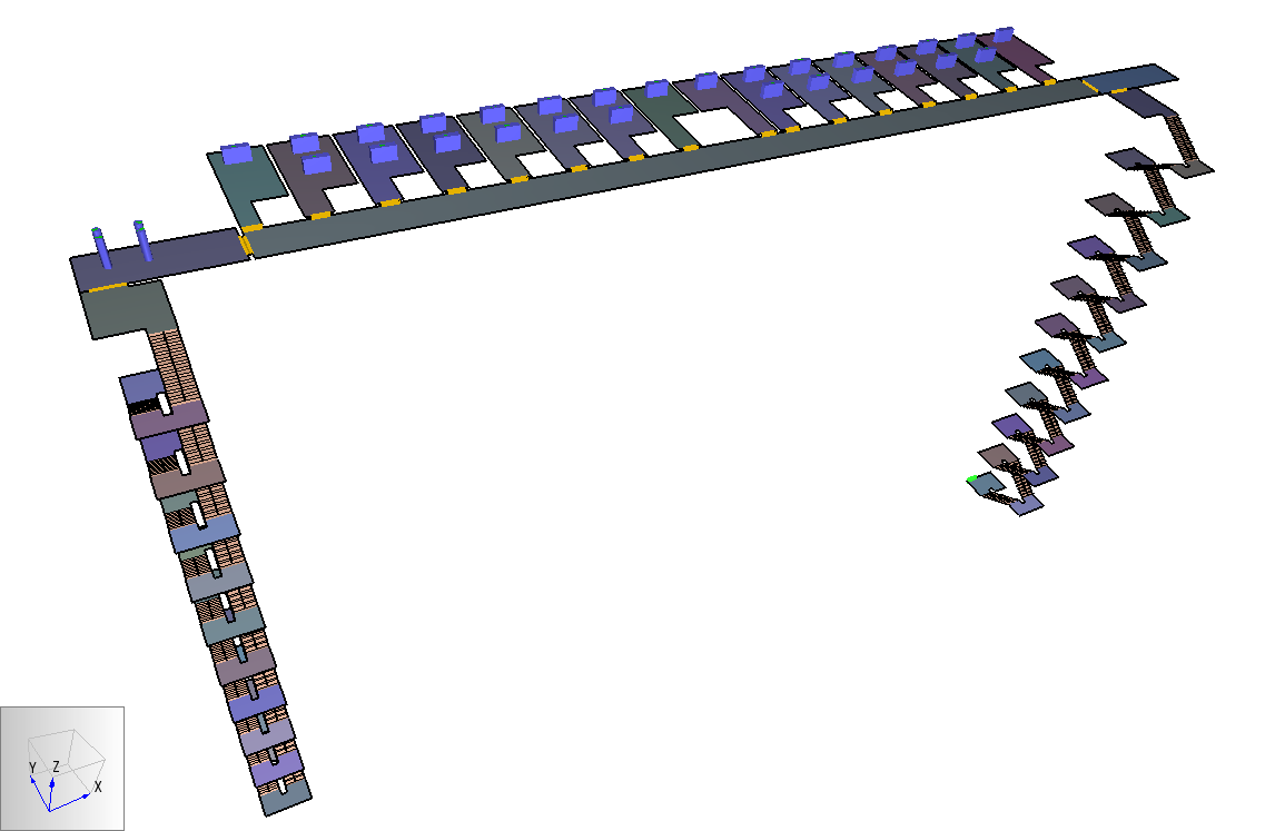
Table 5 gives the speeds for the patients and assistants.
| Role | Horizontal (m/s) | Stair Down (m/s) | Stair Up (m/s) | Initial Delay (s) |
|---|---|---|---|---|
| Stretcher (male team) | 1.09 ±0.08 | 0.63 | N/A | 67.6 |
| Evacuation Chair (female team) | 1.39 ±0.03 | 0.82 | N/A | 35.9 |
| Female and Male Assistants | 1.385±0.055 | 0.885±0.125 | 0.655±0.015 | 0.0 |
Before proceeding to the full evacuation simulation, we first model evacuation of one patient, either in an evacuation chair or stretcher. This allows us to compare to hand calculations.
The first case is one evacuation chair and one female assistant. Table 6 compares results for a hand calculation and Pathfinder (in steering mode and based on nominal speeds given above and distances in the model). The hand calculations do not include any factors such as delay for door opening, cornering speeds, or fatigue. The Pathfinder calculations do include delays and extra movement due to cornering and, as a result, are slower than the hand calculation. For SFPE mode, the stair speeds use the SFPE stair speed factor.
| Evacuation Phase | Steering Mode | SFPE Mode | ||||
| Speed (m/s) | Distance | Time (s) | Speed (m/s) | Distance | Time (s) | |
| Assistant to Patient | 1.385 | 25.9 | 18.7 | 1.385 | 25.9 | 18.7 |
| Preparation | 0.0 | 35.9 | 0.0 | 35.9 | ||
| Patient to Stairs | 1.390 | 34.5 | 24.8 | 1.390 | 34.5 | 24.8 |
| Patient down 20 runs of stairs | 0.820 | 76.4 | 93.1 | 1.070 | 76.4 | 71.4 |
| Patient on 20 landings | 1.390 | 46.0 | 33.1 | 1.390 | 46.0 | 33.1 |
| Patient on bottom landing | 1.390 | 2.4 | 1.7 | 1.390 | 2.4 | 1.7 |
| Assistant on bottom landing | 1.385 | 2.4 | 1.8 | 1.385 | 2.4 | 1.8 |
| Assistant up 20 runs of stairs | 0.655 | 76.4 | 116.6 | 1.070 | 76.4 | 71.4 |
| Assistant on 20 landings | 1.385 | 43.8 | 31.6 | 1.385 | 43.8 | 31.6 |
| Assistant return to start | 1.385 | 7.9 | 5.7 | 1.385 | 7.9 | 5.7 |
| Hand calculation single trip totals: | 315.6 | 363.0 | 315.6 | 296.1 | ||
| Pathfinder: | 407.53 | 302.11 | ||||
The second case is one stretcher with four male assistants. Again, we compare hand calculations with Pathfinder, Table 7. As before, the Pathfinder calculations are slower than the hand calculation. In this case there is additional difficulty maneuvering the stretcher through doors and on the landings. For SFPE mode, the stair speeds use the SFPE stair speed factor.
| Evacuation Phase | Steering Mode | SFPE Mode | ||||
| Speed (m/s) | Distance | Time (s) | Speed (m/s) | Distance | Time (s) | |
| Assistant to Patient | 1.385 | 25.9 | 18.7 | 1.385 | 25.9 | 18.7 |
| Preparation | 0.0 | 67.6 | 0.0 | 67.6 | ||
| Patient to Stairs | 1.090 | 34.5 | 31.7 | 1.090 | 34.5 | 31.7 |
| Patient down 20 runs of stairs | 0.630 | 76.4 | 121.2 | 0.840 | 76.4 | 90.9 |
| Patient on 20 landings | 1.090 | 46.0 | 42.2 | 1.090 | 46.0 | 42.2 |
| Patient on bottom landing | 1.090 | 2.4 | 1.8 | 1.385 | 2.4 | 1.8 |
| Assistant on bottom landing | 1.385 | 2.4 | 1.8 | 1.385 | 2.4 | 1.8 |
| Assistant up 20 runs of stairs | 0.655 | 76.4 | 116.6 | 1.070 | 76.4 | 71.4 |
| Assistant on 20 landings | 1.385 | 43.8 | 31.6 | 1.385 | 43.8 | 31.6 |
| Assistant return to start | 1.385 | 7.9 | 5.7 | 1.385 | 7.9 | 5.7 |
| Hand calculation single trip totals: | 315.7 | 439.3 | 315.7 | 363.7 | ||
| Pathfinder: | 534.0 | 457.63 | ||||
Two scenarios were used for the evacuation of all occupants on the floor:
In the hospital, the day shift team consists of seven assistants. Preparation for evacuation using the evacuation chair requires two assistants but only one assistant is needed during evacuation movement of the chair. To represent this, the simulation for the evacuation chair assumed that one assistant was always occupied with helping prepare occupants and that only six assistants participated in the evacuation movement. For the night shift there are only four assistants and each stretcher requires four assistants during evacuation.
Table 8 summarizes the calculated results. The hand calculation was based on calculations shown in Table 6 and Table 7.
| Simulation | Steering Mode | SFPE Mode | Pathfinder Steering+SFPE (hr) | Exodus (hr) | ||
| Pathfinder (hr) | Hand Calculation (hr) | Pathfinder (hr) | Hand Calculation (hr) | |||
| Evac chair, female team, 6 assistants | 0.53 | 0.46 | 0.39 | 0.38 | 0.54 | 0.6 |
| Stretcher, male team, 4 assistants | 4.17 | 3.37 | 3.61 | 2.80 | 4.27 | 3.8 |
The results are consistent with the hand calculation, in that all Pathfinder calculations are slightly longer than the hand calculations. The SFPE results are shorter than the Steering results primarily because the stair speeds down and up use the faster SFPE stair speed factors. The results are also similar to the Exodus results.
This tests the flow rates of occupant sources. Sources can be used to introduce new occupants into a simulation.
Sources can be assigned to: a rectangular area, rooms, and doors (both internal and exit).
Source parameters include: flow rate (constant or periodic), the profile distribution, the behavior of occupants, and an option to either delay introducing occupants into a crowded room or to enforce the flow rate (even if that will result in overlapping occupants).
The model is shown in Figure 108.
Four source types were tested: rectangle, door, exit door, and room.
The occupants were distributed uniformly between two profiles (red and blue).
The source flowrate is constant at 2.5 pers/s.
The Enforce Flowrate option was selected.
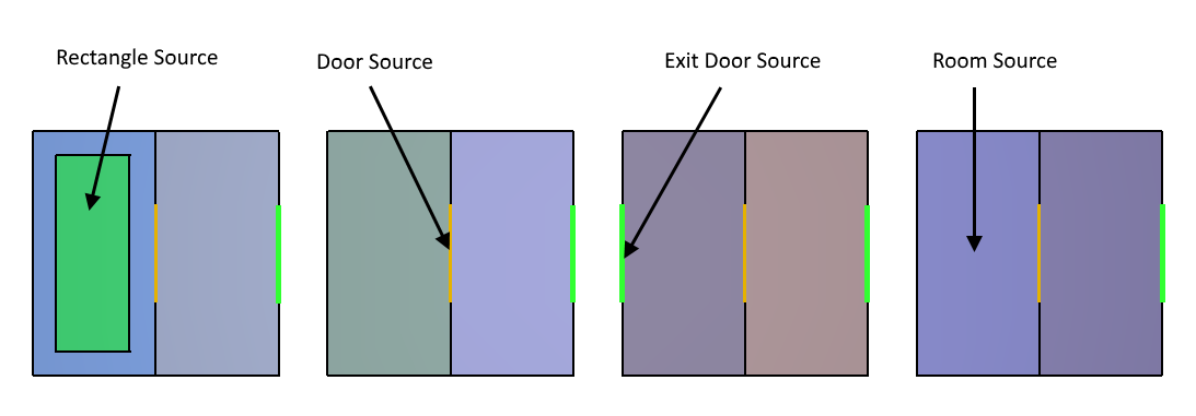
Figure 109 shows the exit door flow rates for the four cases.
In all cases, the flow reaches a steady-state value of 2.5 pers/s.
Results for steering behavior (shown), SFPE and Steering+SFPE are similar.
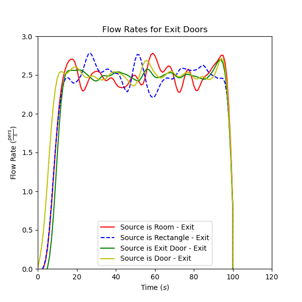
The Pathfinder calculations performed as expected.
The Pathfinder calculation of Fractional Effective Dose (FED) uses the equations described in the SFPE Handbook of Fire Protection Engineering, pages 2308-2428 (SFPE 2016).
The implementation is the same as used in FDS+EVAC (Korhonen 2018), using only the concentrations of the asphyxiant gases \(CO\), \(CO_{2}\), and \(O_{2}\) to calculate the FED value.
\(\text{FED}_{\text{tot}} = \text{FED}_{\text{CO}} \times \text{VCO}_{2} + \text{FED}_{O_{2}}\)
This calculation does not include the effect of hydrogen cyanide (HCN) and the effect of \(CO_{2}\) is only due to hyperventilation.
See the Pathfinder User Manual and Technical Reference Manual for more details.
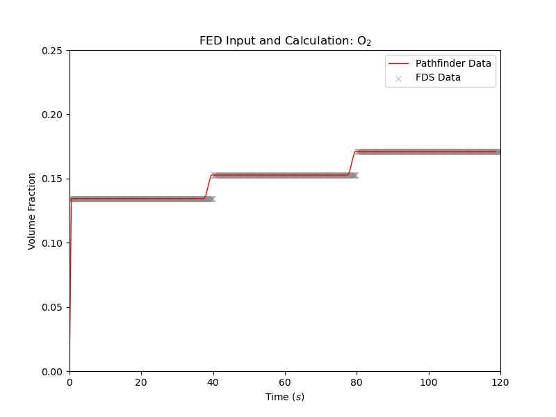
This validation problem tests the calculation of FED for a stationary occupant. The PyroSim model is shown in Figure 110. The model includes a fire and devices that measure the volume fractions of \(CO\), \(CO_{2}\), and \(O_{2}\) at the location of the height of the occupant. The model also uses FDS to calculate FED which is compared to the Pathfinder calculation.
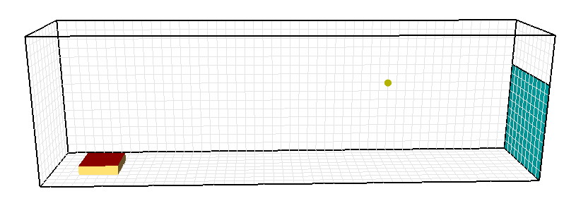
The Pathfinder model is shown in Figure 111.
Pathfinder samples FED quantities at 90% of occupant height.
The default height is 1.8288 m, so devices are located at a height of 1.6459 m in the PyroSim model.
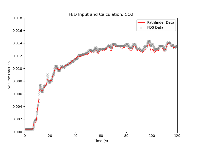
Comparisons of the FDS device outputs and the Pathfinder inputs and calculated FED are shown in Figure 112, Figure 113, Figure 114, and Figure 115. Pathfinder reads 3D Plot data and then interpolates, so there is some difference between the device and interpolated values for \(CO_{2}\), \(CO\), and \(O_{2}\).
 |  |
 | 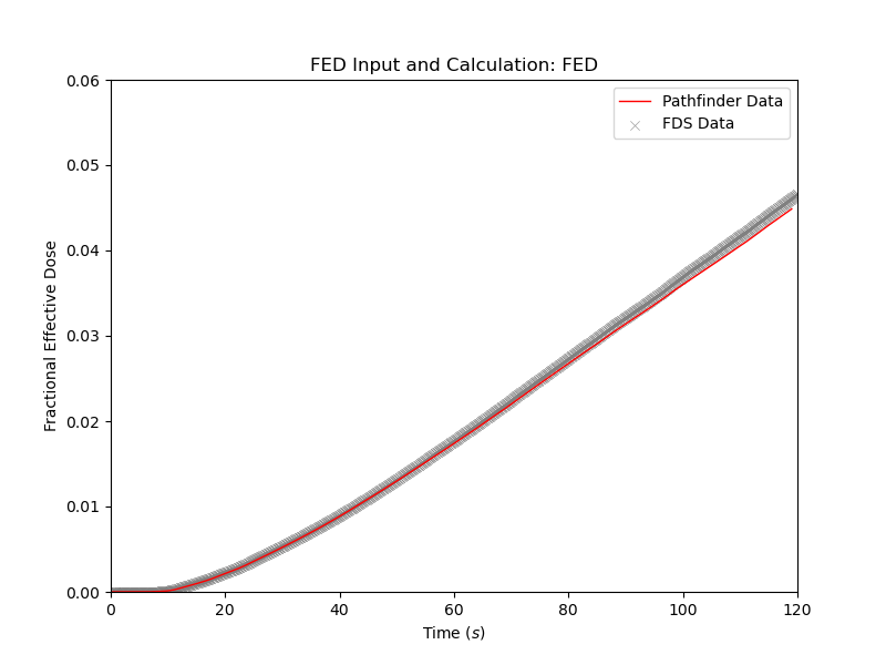 |
As noted, the 3D Plot data output from FDS is somewhat different from the device output.
In addition, the 3D Plot data was output at a time interval of 0.5 seconds, so the FED time integration results in some difference with the FDS device value integrated at a finer time step.
The final values are FED=0.0467 for FDS and FED=0.0455 for Pathfinder (3% difference).
The Pathfinder results are satisfactory.
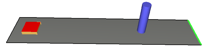
This validation problem tests the calculation of FED for a moving occupant. The PyroSim model is shown in Figure 116. The model is divided into three initial (INIT) regions separated by thin wall obstructions.
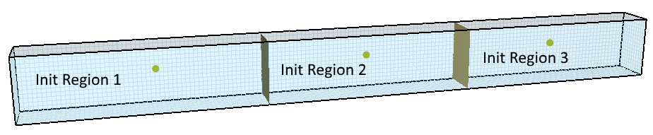
The init regions used a mix of air and combustion products.
The mass fractions of species in the two mixtures are shown in Table 9.
Init Region 1 has 100% mass fraction combustion products, Init Region 2 has 75% combustion products and 25% air, and Init Region 3 has 50% combustion products and 50% air.
| Species | Combustion Products | AIR |
|---|---|---|
| Carbon Dioxide | 0.010000 | 0.000592 |
| Carbon Monoxide | 0.001000 | 0.000000 |
| Nitrogen | 0.839000 | 0.763018 |
| Oxygen | 0.150000 | 0.231164 |
| Water Vapor | 0.000000 | 0.005226 |
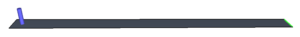
The Pathfinder model is shown in Figure 117.
The occupant starts on the left and has a velocity of 0.25 m/s.
The distance to the exit is 30 m, so the time to exit is approximately 120 seconds (there is some acceleration time at the start).
As the occupant moves through the model, they are exposed to the different gas mixtures.
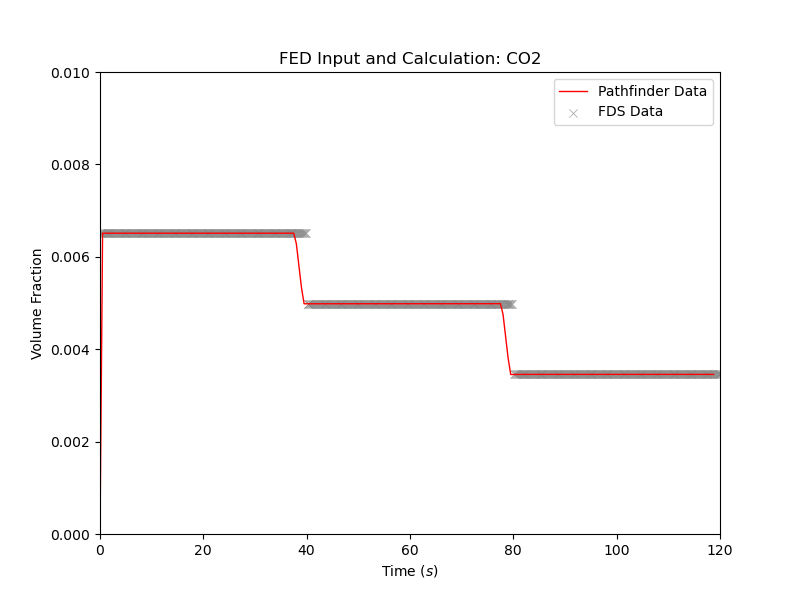
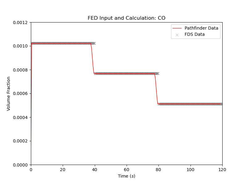
Comparisons of the FDS device outputs and the Pathfinder inputs and calculated FED are shown in Figure 118, Figure 119, Figure 120, and Figure 121. The data shows how the occupant is exposed to different concentrations as they move through the model.
 |  |
 |  |
For this simulation, the concentrations are constant over each initial region.
We can calculate the expected FED by hand to be 0.07896.
Pathfinder calculates 0.07745, a difference of 1.9%. As can be seen in Figure 121, the Pathfinder interpolation of the 3D Plot data leads to a smoothing of the data at the region boundaries.
The Pathfinder results are satisfactory.
The Pathfinder calculation of speed reduction due to smoke is based on a paper by Fridolf, Nilsson, Ronchi, and Frantzich (2019). The walking speed reduction factor \(w_{f}\) is a function of visibility x (m) as shown in Figure 122. The equation for the reduction factor is given by:
The maximum walking speed of the occupant is reduced by the walking speed reduction factor.

To use this feature, it is necessary to first run a PyroSim simulation that calculates visibility. The visibility data is then imported into Pathfinder. The data is extracted for each occupant at their X-Y location and a Z height of 90% of the occupant height. See the Pathfinder User Guide and Pathfinder Technical Reference for more details.
This validation problem tests speed reduction for occupants as they move through different visibilities.
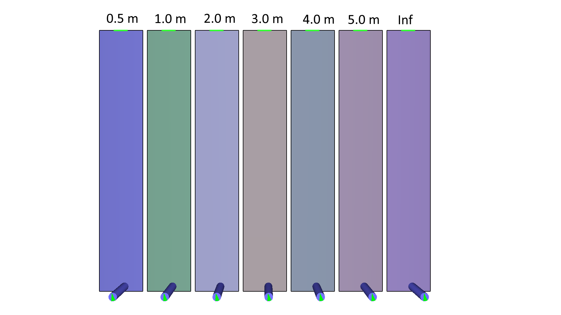
The PyroSim model consists of separated regions where the soot mass fraction is defined to give visibilities of 0.5 m, 1.0 m, 2.0 m, 3.0 m, 4.0 m, 5.0 m, and \(\infin\) m.
The Pathfinder model is shown in Figure 123. Each room has a uniform visibility that results from the soot density.
A comparison of the calculated and expected speeds is shown in Figure 124.
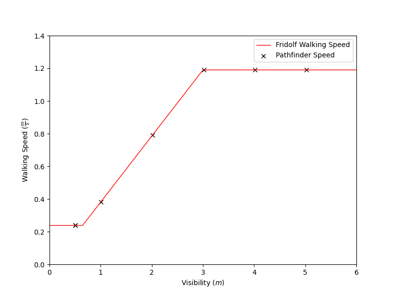
The speeds in smoke calculated by Pathfinder are correctly calculated. The Pathfinder results are satisfactory.
This section presents test cases described in Annex 3 of IMO 1533 (IMO 2016).
This test case verifies movement speed in a corridor for a single occupant.
The test case is based on Test 1 given in Annex 3 of IMO 1533 (IMO 2016).
The test case describes a corridor 2 meters wide and 40 meters long containing a single occupant.
The occupant must walk across the corridor and exit. The occupant’s waking speed is 1.0 m/s.
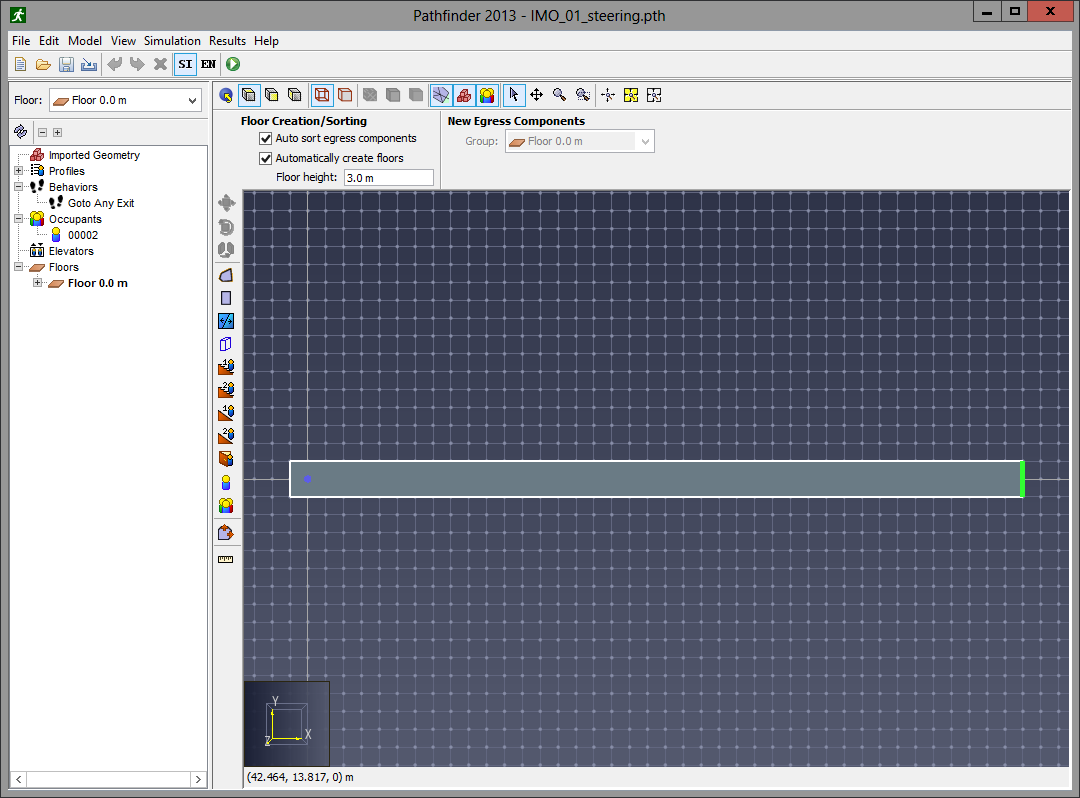
Since Pathfinder tracks occupant location by the center point, the navigation mesh was extended 0.5 meters behind the occupant to allow space for the back half of the occupant when standing exactly 40 meters from the exit.
SFPE mode should give an exit time of 40.0 seconds.
Steering mode uses inertia and we need to account for the time it takes to accelerate to 1.0 m/s.
Occupants in Pathfinder can accelerate to maximum speed in 1.1 s.
From \(d_{1} = 0.5 * (v_{1} - v_{0}) * t_{1}\) we know that with \(v_{0} = 0.0\ m/s\), \(v_{1} = 1.0\ m/s\), at t=1.1 s the occupant will have travelled 0.55 m. The remaining 39.45 meters will be covered at 1.0 m/s. Thus, steering mode should give an exit time of 40.55 seconds.
Table 10 shows the time to exit in each tested mode.
| Mode | Time |
|---|---|
| Steering | 40.55 |
| Steering + SFPE | 40.55 |
| SFPE | 40.02 |
All test cases were successful.
This test verifies movement speed up a stairway for a single occupant.
The test case is based on Test 2 given in Annex 3 of IMO 1533 (IMO 2016).
The test case describes a stairway 2 meters wide and 10 meters long (along the incline).
A single occupant with a maximum walking speed of 1.0 m/s begins at the base of the stairway and walks up to the exit.
This example uses 7"x11" stairs.
The occupant was positioned on a lower landing at a distance 1.0 m from the staircase.
For the steering mode this allows the occupant enough distance to accelerate to full speed before reaching the stairway.
Pathfinder summary file reports the time of the first person entering a stairway and the time the last person leaves, so this provides an accurate measure of time on the stairs for a single occupant.
The occupant is given a base maximum speed of 1.0 m/s.
The default Pathfinder assumption is to use the SFPE stair speed factors.
This speed reduction will be used in all modes with the scaling factor based on the slope of the stairway.
Using the velocity equations presented in the Pathfinder Technical Reference, this scale factor will be (0.918 m/s) / (1.19 m/s) = 0.77.
This makes the effective stairway speed of the occupant (1.0 m/s)*0.77 = 0.77 m/s.
Based on this speed, the results for all modes should be the same at 12.99 s.
Table 11 shows the time to ascend the staircase in each mode (i.e. the stair exit time minus the stair entry time).
| Mode | Time |
|---|---|
| Steering | 12.92 |
| Steering + SFPE | 13.02 |
| SFPE | 12.95 |
All test results are within an acceptable margin of error.
This test case verifies movement speed down a stairway for a single occupant.
The test case is based on Test 3 given in Annex 3 of IMO 1533 (IMO 2016).
The test case describes a stairway 2 meters wide and 10 meters long (along the incline).
A single occupant with a maximum walking speed of 1.0 m/s begins at the top of the stairway and walks down to the exit.
This example uses 7"x11" stairs.
The occupant was positioned on the upper landing at a distance 1.0 m from the staircase.
For the steering mode this allows the occupant enough distance to accelerate to full speed before reaching the stairway.
The length between the occupant’s center starting position and the bottom of the staircase is slightly less than 10.0 m, since at the top of the stairs an occupant must allow for the door tolerance.
The occupant is given a base maximum speed of 1.0 m/s.
The default Pathfinder assumption is to use the SFPE stair speed factors.
This speed reduction will be used in all modes with the scaling factor based on the slope of the stairway.
Using the velocity equations presented in the Pathfinder Technical Reference, this scale factor will be (0.918 m/s) / (1.19 m/s) = 0.77.
This makes the effective stairway speed of the occupant (1.0 m/s) * 0.77 = 0.77 m/s.
Based on this speed, the results for all modes should be the same at 12.99 s.
Table 12 shows the time to descend the staircase in each tested mode (i.e. the stair exit time minus the stair entry time).
| Mode | Time |
|---|---|
| Steering | 12.92 |
| Steering + SFPE | 12.98 |
| SFPE | 12.94 |
All test results are within an acceptable margin of error.
This case verifies the flow rate limits imposed by doorways in the SFPE modes. Results from the steering mode are included for comparison. The test case is based on Test 4 given in Annex 3 of IMO 1533 (IMO 2016). The test case describes a room 8 meters by 5 meters with a 1 meter exit centered on the 5 meter wall. The room is populated by 100 occupants with the expectation that the average door flow rate over the entire period does not exceed 1.33 persons per second.
Flow rate is measured using the simulation summary data. This average flow rate is defined as the number of occupants to pass through a door divided by the amount of time the door was "active." A door is considered to be active after the first occupant has reached the door and is no longer active when the last occupant has cleared the door.
Following SFPE guidelines, the boundary layer for all modes was 15 cm. With this boundary layer, the expected door flow rate for SFPE mode is 0.92 pers/s.
The maximum observed flow rate should be less than 1.33 persons per second.
Table 13 shows the average exit door flow rates observed in each tested mode.
| Mode | Time |
|---|---|
| Steering | 1.04 |
| Steering + SFPE | 0.84 |
| SFPE | 0.93 |
The Steering+SFPE mode shows a slower exit door flow rate, due to the combination of steering movement and door flow rate limits. All test results are within an acceptable margin of error.
This case verifies initial delay (pre-movement) times. The test case is based on Test 5 given in Annex 3 of IMO 1533 (IMO 2016). The test case describes a room 8 meters by 5 meters with a 1 meter exit centered on the 5 meter wall. The room is populated by 10 occupants with uniformly distributed response times ranging from 10 to 100 seconds. Figure 129 shows the initial problem setup. 10 occupants were added to the room at random locations.
Occupants were assigned initial delays between a min = 10.0s and max = 100.0s.
Occupant parameters were not randomized between simulations. This should lead to similar occupant count graphs.
Initial movement times should vary between occupants. This was verified by viewing the results animation. Pathfinder also has the option to output detailed comma-separated files for each occupant.
Results for this problem were first verified using the animation. Results were also verified by examining the output in the detailed output data for each occupant.
All simulator modes passed the test.
The test case is based on Test 6 given in Annex 3 of IMO 1533 (IMO 2016). The test case describes 20 occupants navigating a corner in a 2 meter wide corridor. The expected result is that the occupants round the corner without penetrating any model geometry.
20 persons are uniformly distributed in the first 4 meters of the corridor.
Each occupant should navigate the model while staying inside the model boundaries. For the steering modes the occupants will retain a separation distance, but the SFPE mode allows multiple occupants to be located at the same space.
Figure 131, Figure 132, and Figure 133 show the occupant trails for all 3 simulator modes. These movement trails can be used to verify that all occupants successfully navigated the corner.
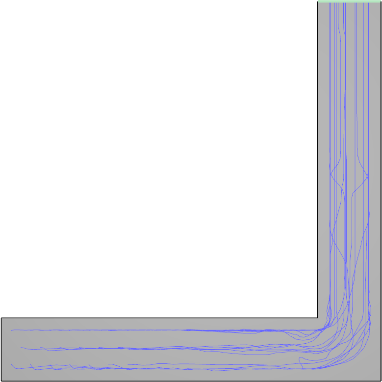 | 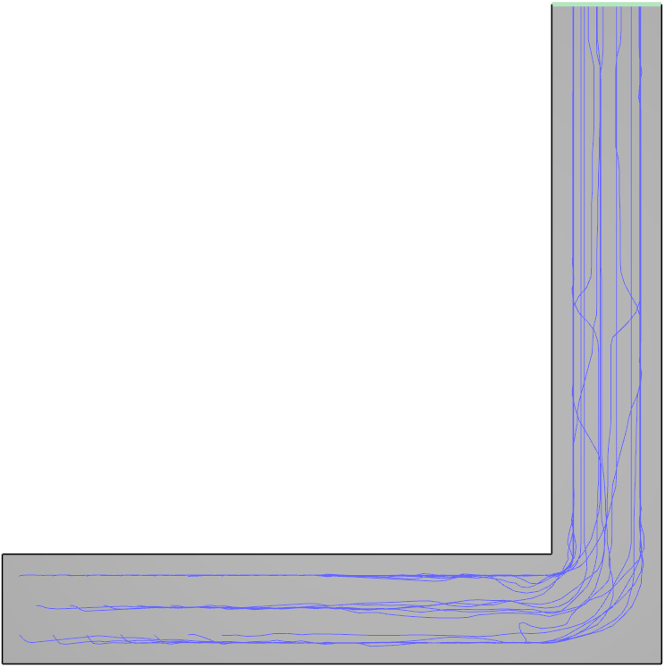 |
 |  |
Occupant trails indicate that no occupants passed outside the simulation boundary in any of the three simulation modes. All simulation modes successfully pass the verification test. The SFPE mode is basically a flow calculation, so occupants may be superimposed in the same space. The steering mode provides the most realistic movement.
All simulator modes passed the test.
This test verifies multiple walking speeds in Pathfinder. The test case is based on Test 7 given in Annex 3 of IMO 1533 (IMO 2016). The test case involves the assignment of population demographics to a group of occupants.
A walking speed profile representing males 30-50 years old is distributed across 50 occupants.
The walking speeds are a uniform random distribution with a minimum of 0.97 m/s and a maximum of 1.62 m/s.
The information for this profile comes from Table 3.4 in the appendix to the Interim Guidelines for the advanced evacuation analysis of new and existing ships.
The occupants were positioned in a line 0.5 m from the left side of a 40.5 x 51.0 m room.
The exit door is on the opposite side of the room.
Each occupant moves with their assigned speed in a straight line to the right.

The occupants should display a range of walking speeds within the specified limits, so that the arrival times at the right edge of the room should be between 24.7 s and 41.2 s (neglecting the inertia in the steering mode).
The occupants' speeds observed in the simulation were within the specified limits. The first arrival and last arrival times at the exit are given in the table below. Figure 136 shows the occupant paths at 20 s for steering mode (other cases are similar).
| Mode | First Arrival (s) | Last Arrival (s) |
|---|---|---|
| Steering | 25.35 | 41.92 |
| Steering + SFPE | 25.35 | 41.92 |
| SFPE | 24.82 | 40.95 |

All simulator modes passed.
This test verifies Pathfinder’s counterflow capability. The test case is based on Test 8 given in Annex 3 of IMO 1533 (IMO 2016). The test case involves the interaction of occupants in counterflow. Two 10 meter square rooms are connected in the center by a 10 meter long, 2 meter wide hallway. 100 persons are distributed on the far side of one room as densely as possible, and move through the corridor to the other room. Occupants in the other room move in the opposite direction. The test is run with 0, 10, 50, and 100 occupants moving in counterflow with the original group.
The problem geometry is set up as described above, with exits at the far walls. The occupants in each room are assigned the exit in the opposite room.
To simplify collection of results, all four simulation scenarios are created in the same model. This can be accomplished by duplicating the initial geometry 3 times, then using different numbers of occupants in the room at the right.
A walking speed profile representing males 30-50 years old is distributed across all occupants.
The walking speeds are a uniform random distribution with a minimum of 0.97 m/s and a maximum of 1.62 m/s.
The information for this profile comes from Table 3.4 in the appendix to the Interim Guidelines for the advanced evacuation analysis of new and existing ships.
As the number of occupants in counterflow increases, the occupants should slow down and increase the evacuation time.
Since in the SFPE mode, there is no restriction on occupants being superimposed in the same space, counterflow does not slow the movement (room density does reduce walking speed for this case).
Figure 138 shows the occupant positions for the steering mode, 100 person counterflow case at 75 s.

Table 15 shows the time it takes occupants that start on the left to exit the simulation on the right. The times are given as a function of the number of occupants in counterflow.
| Number of Occupants Starting on Right Side | ||||
| 0 | 10 | 50 | 100 | |
| Mode | Exit Time Right (s) | |||
| Steering | 67.65 | 78.78 | 143.07 | 220.53 |
| Steering + SFPE | 67.65 | 78.78 | 143.07 | 220.53 |
| SFPE | 29.95 | 30.68 | 31.45 | 33.2 |
In each mode, more counterflow increases evacuation time. The SFPE mode does not account for counterflow interference, the increased times are due to increased room density slowing the speed.
See Fundamental Diagram for Bidirectional Flow for a comparison with experimental data for bidirectional flow.
All modes passed test criteria.
This test verifies Pathfinder’s exit time sensitivity to a changing number of available doors. The test case is based on Test 9 given in Annex 3 of IMO 1533 (IMO 2016). The test case involves the evacuation of 1000 occupants from a large room, 30 meters by 20 meters, with doors of 1.0 m width. The 1000 occupants are distributed uniformly in the center of the room, 2 meters from each wall. The test is run with 4 exits and 2 exits, with the expectation that the evacuation time will double in the 2 exit case.
Occupants are given a profile corresponding to males 30-50 years old from Table 3.4 in the appendix to IMO 1238 (IMO 2016).
The walking speeds are a uniform random distribution with a minimum of 0.97 m/s and a maximum of 1.62 m/s.
To simplify data collection, both model configurations are added to a single simulation model.
Simulation time should approximately double when using half as many doors.
For the SFPE mode, the expected single door flow rate is 0.924 pers/s (15 cm boundary included), giving an evacuation time of 541 s for two doors and 271 s for four doors.
Table 16 shows the time it takes to exit the simulation for both cases. Since the initial locations of the occupants were randomly assigned, the number of persons that exit each door are not exactly equal.
| Model | 4 Doors | 2 Doors | ||
| Min (s) | Max (s) | Min (s) | Max (s) | |
| Steering | 203.18 | 211.43 | 409.90 | 413.30 |
| Steering + SFPE | 283.04 | 295.06 | 578.17 | 582.51 |
| SFPE | 264.77 | 275.60 | 540.68 | 549.33 |
For all modes, the simulation times, while not exactly double, are well within the acceptable margin for validity.
All modes passed test criteria.
This test verifies exit assignments in Pathfinder. The test case is based on Test 10 given in Annex 3 of IMO 1533 (IMO 2016). 23 occupants are placed in a series of rooms representing ship cabins and assigned specific exits.
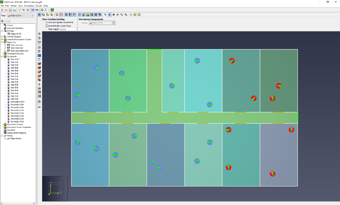
The occupants in the left 8 rooms are assigned to the main (top) exit.
The occupants in the remaining 4 rooms are assigned to the secondary (right) exit.
Occupants are given a profile corresponding to males 30-50 years old from Table 3.4 in the appendix to IMO 1238 (IMO 2016).
The walking speeds are a uniform random distribution with a minimum of 0.97 m/s and a maximum of 1.62 m/s.
Each occupant should leave the model using the specified exit.
Figure 141 shows the paths taken by occupants in steering mode (other modes were similar). The trails of the four occupants intended to use the secondary exit are shown in red, all other occupant trails are shown in blue.
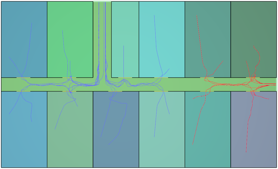
The results for all simulator modes indicate that the four occupants directed to exit via the secondary exit, did so.
All modes passed test criteria.
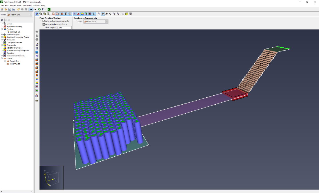
This test examines the formation of congestion in Pathfinder. The test case is based on Test 11 given in Annex 3 of IMO 1533 (IMO 2016). 150 occupants must move from a 5 m x 8 m room, to a 2 m x 12 m corridor, up a stairway, and out of the simulation via a 2 m wide platform. Congestion is expected to form initially at the entrance to the corridor, then later at the base of the stairs.
Figure 142 shows the problem setup in Pathfinder. The red rectangle indicates the region used to measure density.
A specific definition for congestion is given in Section 3.7 of IMO 1533 (IMO 2016).
Congestion is present when either of the following conditions is achieved: initial density is at least 3.5 pers/m2, or queues grow (occupants accumulate) at a rate of more than 1.5 pers/s at a joint between two egress components.
The initial density in the 5m x 8m room containing 150 occupants is 3.75 pers/m2.
Based on the congestion criteria, this condition is sufficient to qualify the initial room as congested.
Congestion is measured using the queue at the base of the stairway.
Congestion is identified by either of the following criteria: (1) initial density equal to, or greater than, 3.5 persons/m2; or (2) significant queues (accumulation of more than 1.5 persons per second between ingress and exit from a point).
The 150 occupants are added to the initial room using a uniform distribution.
All occupants were assigned a profile corresponding to 30-50 year old males (as specified in Table 3.4, International Maritime Organization, 2016).
On level terrain (corridor), this gives a uniform speed distribution ranging from 0.97 m/s to 1.62 m/s (mean 1.3 m/s).
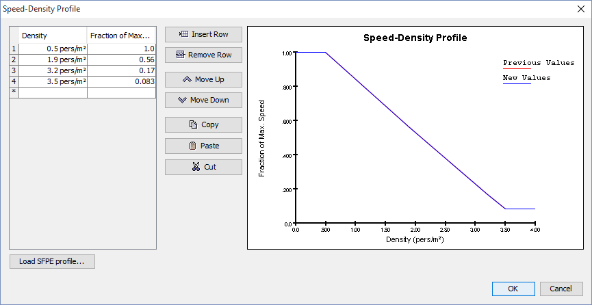
Table 1.1 of the IMO report gives the speed-density curve to be used in calculations.
For a corridor, at a density of 0.5 pers/m2 the speed is 1.2 m/s and at a density of 3.5 pers/m2 the speed is 0.1 m/s.
The corresponding normalized speed-density profile is shown in Figure 143.
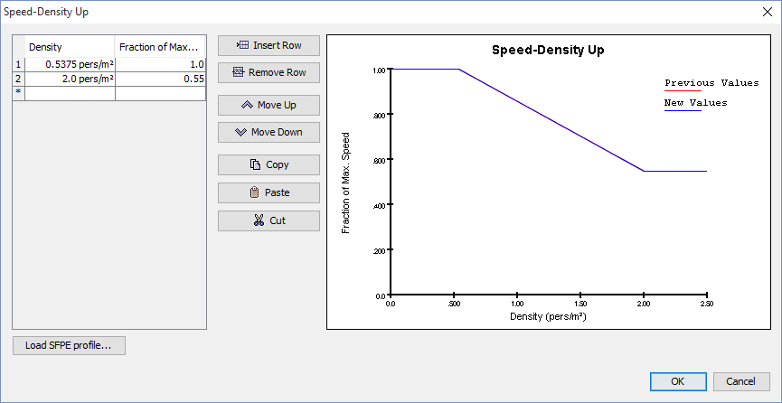
When walking up on stairs, the speed is a uniform speed distribution ranging from 0.47 m/s to 0.79 m/s (mean 0.63).
Table 1.3 of the IMO report gives specific flow and speed curves to be used on stairs up.
At a density of 0.5375 pers/m2 the speed is 0.8 m/s and at a density of 2 pers/m2 the speed is 0.44 m/s.
The corresponding normalized speed-density profile on stairs up is shown in normalized-speed-density.
Congestion should form in the corridor leading to the stairs. This will be measured by the mean density and mean velocity of the occupants in a 2x2 m rectangle at the base of the stairs. The results with and without stairs will be compared.
We can estimate the fastest exit time for the SFPE case.
For a walking speed of 1.62 m/s, the time to cross the 12 m corridor is 7.4 s (neglecting inertia).
The length of the stairs is 5.7 m, so for a 50% speed decrease on stairs, the time required is 7.0 s.
Crossing the landing requires another 1.2 s, for a total of time of 15.6 s.
The total evacuation times for the three cases are given in Table 17.
| Mode | First Out (s) | Last Out (s) |
|---|---|---|
| Steering | 17.00 | 153.70 |
| Steering + SFPE | 17.48 | 156.70 |
| SFPE | 17.90 | 160.90 |
Figure 145 visually shows congestion forming at the base of the stairs.
The density contour shows densities of about 2.75 pers/m2 at the base of the stairs.

Time history data describing the mean density and walking speeds for the occupants at the base of stairs with and without stairs are shown in Figure 146 and Figure 147.
Without stairs, the occupants continue moving to the exit with a speed of about 1 m/s and the maximum density is about 1.25 pers/m2.
With stairs, congestion forms leading to a maximum density of about 3.0 pers/m2 and the speed drops to about 0.25 m/s.
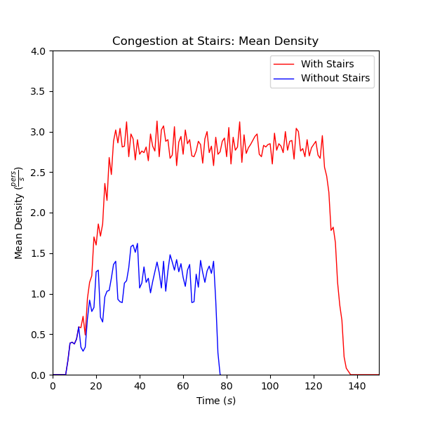 | 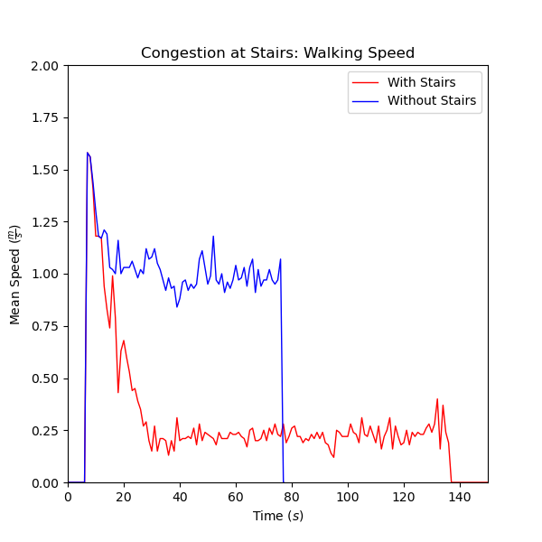 |
Congestion forms at the base of the stairs as shown by comparing the mean density and speeds at the base of the stairs for cases with and without stairs.
Because of the assumed fundamental diagram, the maximum density reaches approximately 3.0 pers/m2, not the 3.5 pers/m2 assumed in HMO for congestion.
However, the Pathfinder results show congestion that is consistent with the specified walking speeds and speed-density curves.
This section presents test cases described in NIST Technical Note 1822 (2013). Section 3 (Suggested Verification and Validation Tests) presents a new set of recommended verification tests and discusses possible examples of validation tests. Tests have been presented in relation to the five main core elements available in evacuation models, namely 1) pre-evacuation time, 2) movement and navigation, 3) exit usage, 4) route availability and 5) flow conditions/constraints.
A modification of IMO Test 5, which has already been presented.
IMO Test 1, which has already been presented.
IMO Tests 2 and 3, which have already been presented.
IMO Test 6, which has already been presented.
A modification of IMO Test 7, which has already been presented.
The current version of Pathfinder does not use visibility to change walking speeds, so this verification test is not applicable.
Pathfinder does allow the user to specify a Speed Modifier by room that can be defined as values as a function of time. This can be used to approximate the effect of smoke in a room. See Manually Coupling FDS and Pathfinder to Respond to Smoke.
This test verifies the capability to simulate occupant incapacitation due to the toxic and physical effects of smoke. Pathfinder can calculate FED for occupants, but the FED exposure does not change the behavior of the occupants.
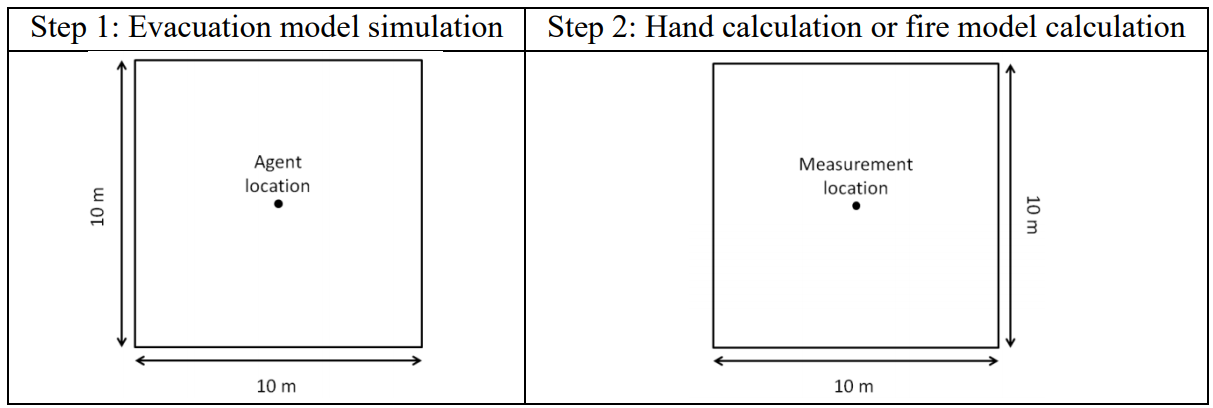
The suggested test, Figure 148, is a room with no fire source (10 m x 10 m x 3m). A stationary occupant is positioned in the room. The room is filled with gas at hazardous conditions consistent with the Fractional Effective Dose (FED) calculation implemented in the software. Comparisons are made with hand calculations or fire model simulation.
Figure 149 shows the Pathfinder model. At the center of the model, devices are used to measure \(CO\), \(CO_{2}\), \(O_{2}\), and the FED value calculated by FDS.

The Pathfinder calculation of Fractional Effective Dose (FED) uses the equations described in the SFPE Handbook of Fire Protection Engineering (5th Edition, Vol 3, Chapter 63, pages 2308-2428). The implementation uses only the concentrations of the asphyxiant gases \(CO\), \(CO_{2}\), and \(O_{2}\) to calculate the FED value.
This calculation does not include the effect of hydrogen cyanide (HCN) and the effect of \(CO_{2}\) is only due to hyperventilation.
See the Pathfinder User Guide and Pathfinder Technical Reference for more details.
Table 18 gives the mass and volume fractions of air and the gas mixture used for the incapacitation calculation. The FED was calculated for air and for the incapacitation case.
| Species | Air | Incapacitation Calculation | ||
| Mass Fraction | Vol Fraction | Mass Fraction | Vol Fraction | |
| N2 | 7.630774E-01 | 7.835682E-01 | 8.270000E-01 | 8.420530E-01 |
| O2 | 2.311814E-01 | 2.078229E-01 | 1.500000E-01 | 1.337080E-01 |
| CO2 | 5.919362E-04 | 3.869034E-04 | 1.000000E-02 | 6.481168E-03 |
| CO | 0 | 0 | 5.000000E-03 | 5.091609E-03 |
| H2O | 5.149269E-03 | 8.222023E-03 | 8.000000E-03 | 1.266627E-02 |
The FED calculation for air should be approximately zero for all time. The FED calculation using the incapacitation gas mixture should increase linearly with time. The time at which FED is equal to one should match the hand calculation and the fire simulator calculation.
At 300 seconds, the FED calculation for pure air was 0.001589.
The small non-zero value is due to the slight difference in default \(O_{2}\) volume fraction assumed in FDS as compared to the value of 20.9 in the SFPE equations.
For the incapacitation calculation, FED = 1 was calculated to occur at 247.5 seconds. The hand calculation gives 247.4. The calculated result matches the expected result.
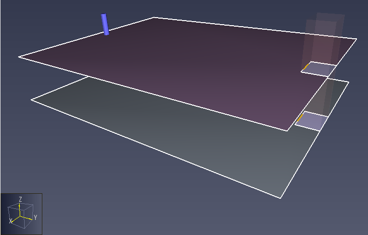
This test verifies the capability of evacuation models to simulate evacuation using elevators. A schematic of the geometry is shown in Figure 150. The corresponding Pathfinder model is shown in Figure 151.
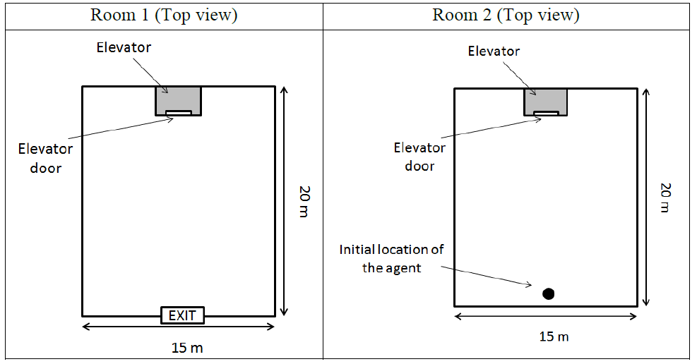
Room 1 is located at Z=0.0 and Room 2 at Z=3.5 m.
An elevator connects the two rooms in accordance with Figure 150.
The Floor 1 exit door is 1 m wide.
The elevator is called from Room 1, reaches Room 2 and carries the occupant and back to Room 1.
The occupant has an unimpeded walking speed of 1 m/s in Room 2 with an instant response time.
To minimize inertia effects, the Acceleration Time was set to zero.
To simplify distance calculations, the occupant size was set to 50 cm.
The initial distance between the center of the occupant and the elevator door is 17.5 m.
However, since the occupant radius is 0.25 m and the distance from the elevator to activate a call is 0.5 m, the occupant walks 16.75 m to activate the call.
The elevator parameters include: door open and close times of 3.5 s, pickup and discharge travel times of 2.5 s between the two floors, and door open and close delays of 5.0 s.
The open delay is the minimum time an elevator’s door will stay open on a floor (does not impact this test case) and the close delay is the time the elevator door will remain open after the last person enters.
The occupant starts walking at time zero and the elevator is called from the discharge floor after the occupant has walked 16.75 m.
Once called, the door must close on the discharge floor and then the elevator must move to the second floor.
The door then opens, the occupant enters the elevator by moving the distance of the occupant radius away from the door (the occupant moves at about a 45° angle), there is a door close delay, and finally the door closes. The elevator then moves to the discharge floor, the door opens, and the occupant leaves the building.
The total expected evacuation time is 60.60 s, shown in Table 19.
| Evacuation Time | ||
|---|---|---|
| Task | Calc | Cumulative Time |
| Start | 0.0 | 0.0 |
| Walk to Activate Elevator Call | 16.75 | 16.75 |
| Door Closes on Discharge Floor | 3.50 | 20.25 |
| Elevator Pickup Time | 2.50 | 22.75 |
| Door Open on Call Floor | 3.50 | 26.25 |
| Load Time | 0.35 | 26.60 |
| Door Close Delay Time | 5.00 | 31.60 |
| Door Close on Call Floor | 3.50 | 35.10 |
| Elevator Discharge Travel Time | 2.50 | 37.60 |
| Door Open on Discharge Floor | 3.50 | 41.10 |
| Building Exit Time | 19.50 | 60.60 |
The observed exit time is 60.5 s for SFPE mode.
Identical results (within tolerance) were obtained for the Steering+SFPE and Steering modes.
All modes passed test criteria.
A modification of IMO Test 8, which has already been presented.
This test verifies movement in a group.
A group (Zone 1) is defined where four members of the group have a walking speed of 1.25 m/s and one member a speed of 0.5 m/s.
In Zone 2, individual occupants have an unimpeded speed of 0.2 m/s.
All occupants proceed to the 1 m wide exit.
The geometry defined in the NIST document and the corresponding Pathfinder model are shown in Figure 152 and Figure 153. In the Pathfinder model, the blue and red occupants are in the group and the center occupant has the slow speed. The green occupants act as individuals.
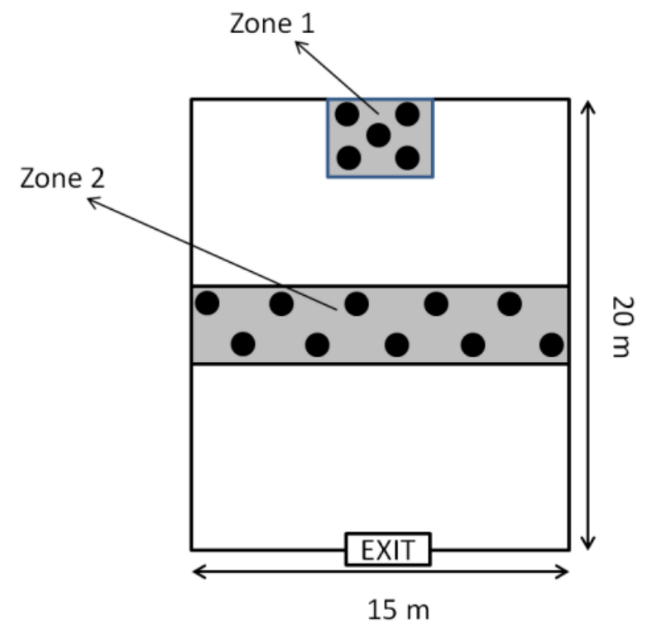
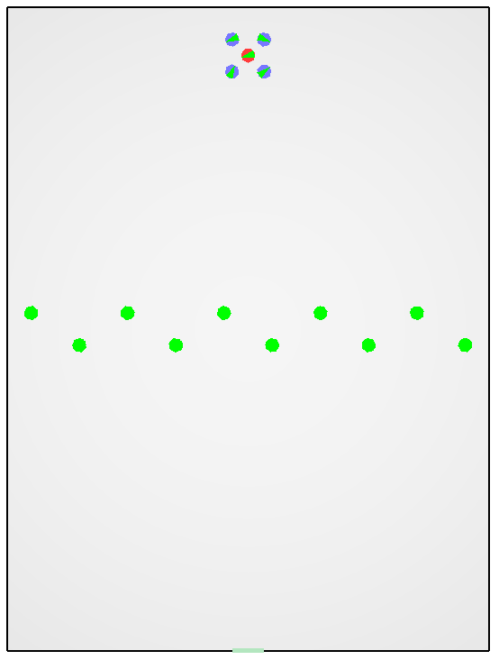
Two parameters in Pathfinder control group behavior: Maximum Distance and Slowdown Time. Members of the group try to maintain a distance between themselves less than the maximum distance. If any member is separated by more than the maximum distance, the leading members slow down for an interval equal to the Slowdown Time. If the group has still not reformed after that time, then the leading members will stop and wait for the group to reform.
Results will be presented using the default Pathfinder parameters that define a relatively loose group, Maximum Distance = 2 m and Slowdown Time = 3 s.
Only results for steering mode are presented because steering+SFPE gives similar results. In SFPE mode occupants can overlap so, as expected, the group just proceeds through the slow occupants without interaction.
The group of five occupants should remain together and exit the door within a time frame of 10 seconds.
Figure 154, Figure 155, and Figure 156 show a sequence of images for default grouping showing movement at 20 s, at 36.5 seconds when the first group member exits, and at 45 seconds when the last group member exits. The time interval for the group to exit is 8.5 seconds.
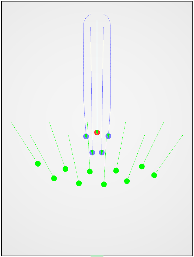 | 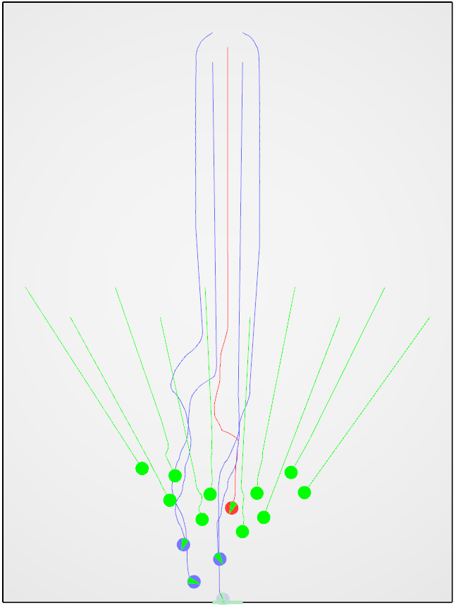 |
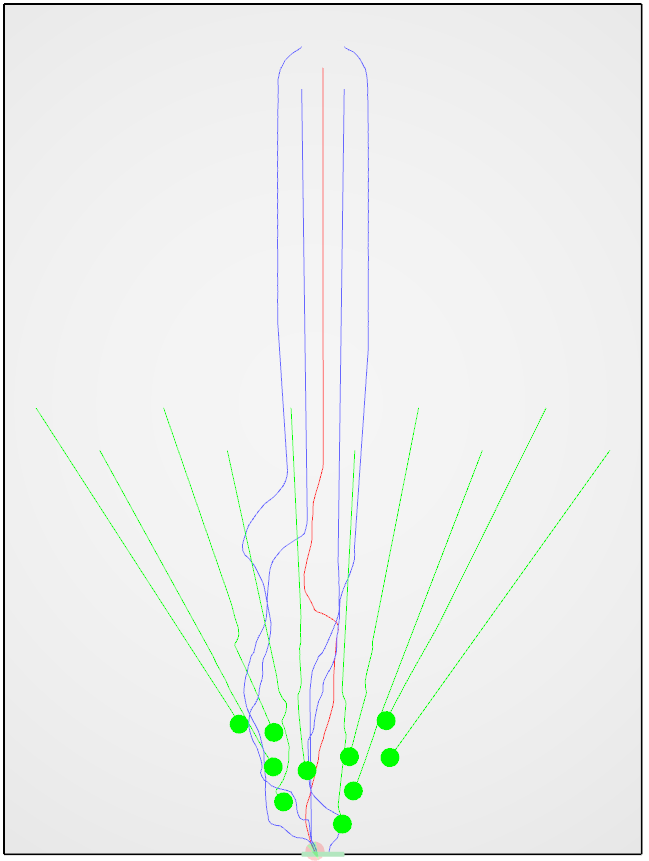 | |
This test is designed for the verification of emerging behaviors of people with disabilities. It tests the possibility of simulating an occupant with reduced mobility (e.g. decreased travel speeds and increased space occupied by the occupants) as well as representing the interactions between impaired individuals and the rest of the population and the environment.
Construct two rooms at different heights, namely room 1 (1 m above the ground level) and room 2 (at ground level), connected by a ramp (or a corridor/stair if the model does not represent ramps). Insert one exit (1 m wide) at the end of room 2.
Scenario 1: Room 1 is populated with a sub-population consisting of 24 occupants in zone 1 (with an unimpeded walking speed of 1.25 m/s and the default body size assumed by the model) and 1 disabled occupant in zone 2 (the occupant is assumed to have an unimpeded walking speed equal to 0.8 m/s on horizontal surfaces and 0.4 on the ramp.
The disabled occupant is also assumed to occupy an area bigger than half the width of the ramp (>0.75 m).
All occupants must reach the exit in room 2.
Scenario 2: Re-run the test and populate zone 2 with an occupant having the same characteristics of the other 24 occupants in zone 1 (i.e. no disabled occupants are simulated). All occupants must reach the exit in room 2.
A schematic of the geometry is shown in Figure 157. The corresponding Pathfinder model is shown in Figure 158.
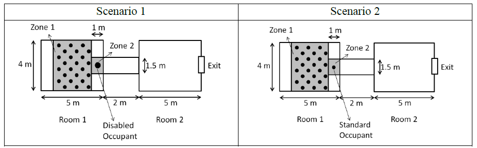
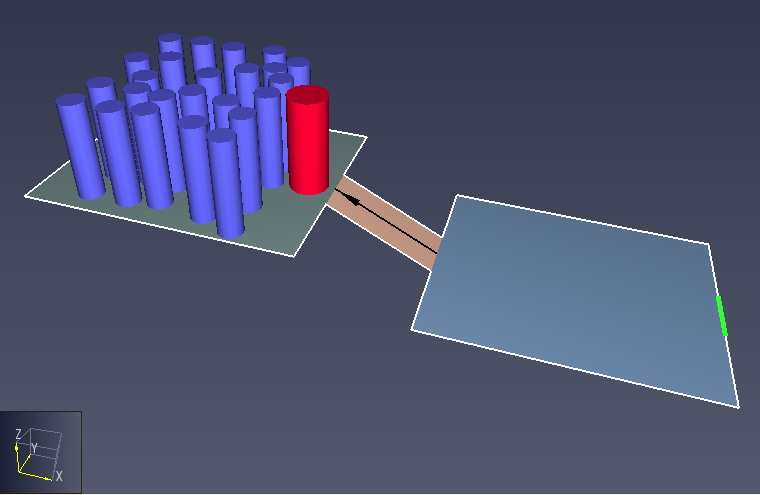
The room geometry is setup as defined.
The shoulder width of the 24 occupants is 45.58 cm and of the disabled person 75 cm.
The walking speed of the 24 occupants is Room 1 is 1.25 m/s and the walking speed of the disabled person was defined as 0.8 m/s.
The disabled occupant was given a ramp speed was 0.4 m/s with other occupants walking the same speed on the ramp and level.
The SFPE and Steering+SFPE calculations included a 15 cm boundary layer.
All occupants will reach the exit. Scenario 1 will have a longer evacuation time than scenario 2.
Table 20 shows the time to evacuate all occupants. The disabled occupant did slow the evacuation slightly by blocking flow on the ramp, but after leaving the ramp the faster occupants moved around the disabled occupant, so the slowing effect was reduced, Figure 159 and Figure 160.
| Mode | Scenario 1 (s) | Scenario 2 (s) |
|---|---|---|
| Steering | 44.58 | 33.62 |
| Steering + SFPE | 48.42 | 40.80 |
| SFPE | 36.10 | 32.70 |
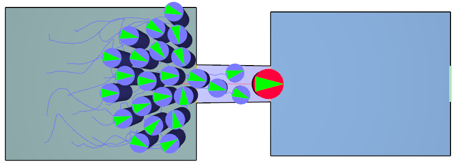
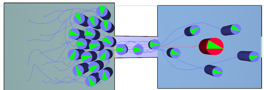
A modification of IMO Test 10, which has already been presented.
The current version of Pathfinder does not use social influence, so this verification test is not applicable.
The current version of Pathfinder does not use social affiliation, so this verification test is not applicable.
This test is aimed at qualitatively evaluating the capabilities of the model to represent the dynamic availability of exits.
Construct a room of size 10 m by 15 m. Two exits (1 m wide) are available on the 15 m walls of the room and they are equally distant from the 10 m long wall at the end of the room (see Figure 161).
Insert an occupant in the room with a response time equal to 0 and a constant walking speed equal to 1 m/s as shown in Figure 161.
Exit 1 becomes unavailable after 1 s of simulation time.
Check the exit usage for both Exit 1 and Exit 2.
A schematic of the geometry is shown in Figure 161.
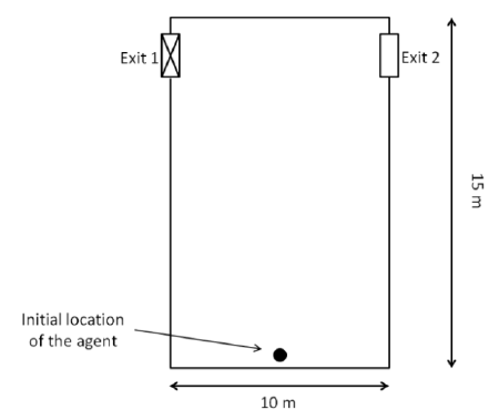
The room geometry is setup as defined.
Pathfinder uses a "locally quickest" algorithm to select the exit door from a room.
To ensure that the occupant selects Exit 1, the occupant was located at X=4.5 m or X=0.5 m closer in the X direction to Exit 1.
The occupant will initially select Exit 1, then at 1.0 s will change to Exit 2.
Figure 162 shows path used by the occupant. At 1.0 s, the occupant changes from Exit 1 to Exit 2. The same result was obtained for Steering+SFPE and SFPE modes.
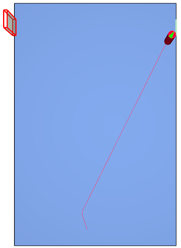
A modification of IMO Test 11, which has already been presented.
A modification of IMO Test 4, which has already been presented.
This section presents Pathfinder results for models based on example problems given for the hand calculations presented in the Engineering Guide for Human Behavior in Fire (SFPE 2019).
This is a verification test for SFPE-based simulation results. This example reproduces Example 1 given in the SFPE Engineering Guide. In this example, 300 occupants are initially positioned in a room of unspecified geometry. The occupants egress through two 32 inch doors that lead to two enclosed 44 inch stairs. The room is connected (directly) to two 44 in wide stairways via two 32 in doors. The occupants must move through the doors and down the 7 x 11 inch (height and depth), 50 ft long stairs. After reaching the base of the stairway, the occupants exit the model through a 30 ft x 6 ft room. The problem specifies that the maximum travel distance between an occupant’s initial position and the nearest door leading to a stairway is 200 ft. This test will assume the initial room is a 200 ft x 30 ft room with both stairways positioned on one of the 30 ft walls Figure 163. The small room is 6 ft x 30 ft with an exit spanning the wall opposite the stairs.
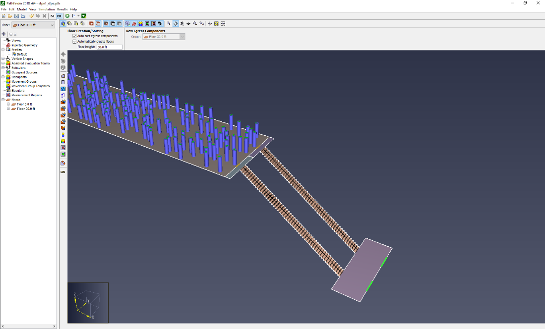
The door boundary layer is specified as 6 in.
In this example, the door entering each stairway is the controlling component. The problem is symmetrical so, for the hand calculation, the divided flow can be modeled as a single wide door and stairway. To calculate the total movement time, we must calculate \(T_{TOTAL} = T_{1} + T_{2} + T_{3}\) where: (\(T_{1}\)) is the time it takes the first occupant to reach the controlling component, (\(T_{2}\)) the time it takes 300 occupants to flow through two 32-inch doors, and (\(T_{3}\)) the time it takes the last occupant to move from the controlling component to the exit.
The value of \(T_{1}\) depends on the location of the occupants. For this model, the value is approximately \(T_{1} = \mathbf{1.0\ s}\).
The time needed for 300 occupants to pass through the two 32 inch doors, \(T_{2}\) is:
The time needed for the last occupant to move down the stairs and out the landing, \(T_{3}\) is:
The total evacuation time, \(T_{total}\) is:
For each simulation mode, Table 21 lists the number of people that used each stair and the total evacuation time. Because the number of people that use the left and right exits are not equal, we present the times for each side.
| Mode | Total Persons - Left | Total Persons - Right | Evacuation Time - Left (s) | Evacuation Time - Right (s) |
|---|---|---|---|---|
| Steering | 152 | 148 | 238.07 | 236.40 |
| Steering + SFPE | 152 | 148 | 273.48 | 274.93 |
| SFPE | 148 | 152 | 239.22 | 245.18 |
All cases show satisfactory comparison with the expected result.
This is a verification test for SFPE-based simulation results. This example reproduces Example 2 given in the SFPE Engineering Guide, (SFPE 2019). In this example, we have a 5-story building. Each floor is served by two 44 inch stairways. The stairs have a 7 inch rise and an 11 inch run. The stairways have hand-rails on both sides 2.5 inches from the wall. Each stairway connects to a 4 ft x 8 ft platform located between the level of the floors. The distance between the floors is 12 ft. The stairways connect to the floors with 32 inch doors. There are 200 people on each floor. Figure 164 shows the problem setup.
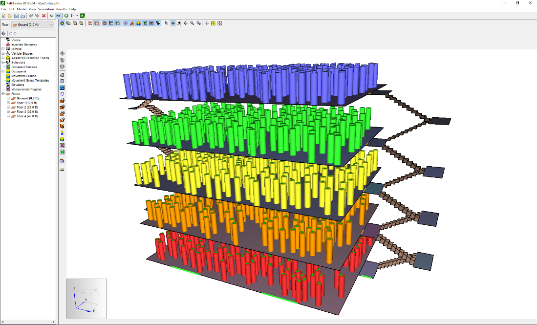
Detailed setup notes are presented in the Pathfinder example guide.
Following the intention of the problem, all occupants of the ground floor exit from four large side doors and all occupants on higher floors exits from doors at the base of the stairs.
A second steering mode case was run where occupants had an increased preference to remain in their current door queue (Current Door Preference parameter of the Profile). This parameter was changed from the default 35% to 80%.
In this example, the controlling component is the exit door at the base of the stairway. We will assume the occupants use the stairways evenly, in which case we only need to model the time it takes for half the occupants on the second through fifth floors to pass through the controlling 32 inch door.
To calculate the total movement time, we must calculate \(T_{TOTAL} = T_{1} + T_{2} + T_{3}\) where:
The calculation for T1 has four parts:
We assume a low-density velocity calculation for the first occupant to reach the stairs and the landing. For \(T_{A}\) we assume the person must walk 6 ft to reach the center of the stairs. For \(T_{B}\) we will assume the occupant must walk 8 ft, an average length of travel, to traverse the platform. This leads to the following calculations:
The time for 400 people to move through a 32 inch door, \(T_{2}\) is:
The time for the last person to move from the stairs to the exit is:
The total evacuation time, \(T_{total}\) is:
For each simulation mode, Table 22 lists the results for both exits, including the number of people that used each exit. When queues form on the upper floors, people waiting in the queues can decide to leave their current queue when another door begins to flow, even if the flow is intermittent. The resulting back and forth behavior, while it does not significantly affect the total exit time, can appear somewhat unexpected. Pathfinder allows the user to increase the commitment of occupants to remain in the queues they are currently in. These are the results reported for the Steering (queue) case.
| Mode | Total Person - Exit 1 | Total Person - Exit 2 | Evacuation Time - Exit 1 | Evacuation Time - Exit 2 |
|---|---|---|---|---|
| Steering | 405 | 395 | 556.35 | 549.73 |
| Steering + SFPE | 403 | 397 | 620.63 | 612.08 |
| SFPE | 409 | 391 | 627.03 | 601.18 |
| Steering (Queue) | 413 | 387 | 563.27 | 539.00 |
The average exit time for the SFPE case matches the expected value within tolerance. The Steering+SFPE case is slower. The Steering mode is faster, since door flow rates are not explicitly specified. Adding the increased commitment to remain in the current queue had the effect of stopping the back and forth movement to alternate queues.
“ISO 16730-1:2015(E) - Fire Safety Engineering — Procedures and Requirements for Verification and Validation of Calculation Methods.” 2015. International Organization for Standardization.
“IEEE 1012-2016 - IEEE Standard for System, Software, and Hardware Verification and Validation.” 2016. Institute of Electrical and Electronics Engineers.
Averill, Jason D., Dennis S. Mileti, Richard D. Peacock, Erica D. Kuligowski, Norman Groner, Guylene Proulx, Paul A. Reneke, and Harold E. Nelson. 2005. “Occupant Behavior, Egress, and Emergency Communication. Federal Building and Fire Safety Investigation of the World Trade Center Disaster (NIST NCSTAR 1-7).” National Construction Safety Team Act Reports (NCSTAR). National Institute of Standards and Technology, Gaithersburg, Maryland, USA. https://www.nist.gov/publications/occupant-behavior-egress-and-emergency-communication-federal-building-and-fire-safety-0.
Boyce, K.E., David Purser, and T. Shields. 2012. “Experimental Studies to Investigate Merging Behaviour in a Staircase.” Fire and Materials 36 (August). https://doi.org/10.1002/fam.1091.
Fridolf, Karl, Enrico Ronchi, Daniel Nilsson, and Håkan Frantzich. 2019. “The Representation of Evacuation Movement in Smoke- Filled Underground Transportation Systems.” Tunnelling and Underground Space Technology 90 (April): 28–41. https://doi.org/10.1016/j.tust.2019.04.016.
Galea, E.R., G. Sharp, and P.J. Lawrence. 2008. “Investigating the Representation of Merging Behavior at the Floor—Stair Interface in Computer Simulations of Multi-Floor Building Evacuations.” Journal of Fire Protection Engineering 18 (4): 291–316. https://doi.org/10.1177/1042391508095092.
Hunt, Aoife, Edwin R. Galea, and Peter J. Lawrence. 2013. “An Analysis and Numerical Simulation of the Performance of Trained Hospital Staff Using Movement Assist Devices to Evacuate People with Reduced Mobility.” Fire and Materials 39 (4): 407–29. https://doi.org/10.1002/fam.2215.
IMO. 2016. “IMO Guidelines for Evacuation Analysis for New and Existing Passenger Ships. MSC.1/Circ.1533.” 4 Albert Embankment, London, Great Britain: International Maritime Organization.
Klote, J. H., and D. M. Alvord. 1992. “Feasibility and Design Considerations of Emergency Evacuation by Elevators.” NISTIR. National Institute of Standards and Technology, Gaithersburg, Maryland, USA, and George Mason University, Fairfax, Virginia, USA. http://bit.ly/3aOfSiJ.
Korhonen, Timo. 2018. Fire Dynamics Simulator with Evacuation: FDS+Evac, Technical Reference and User’s Guide. Sixth Edition. VTT Technical Research Centre of Finland: VTT. http://virtual.vtt.fi/virtual/proj6/fdsevac/documents/FDS+EVAC_Guide.pdf.
SFPE. 2016. SFPE Handbook of Fire Protection Engineering. 5th ed. Springer-Verlag New York. https://www.springer.com/us/book/9781493925643.
———. 2019. SFPE Guide to Human Behavior in Fire. 2nd ed. Springer International Publishing. https://www.springer.com/gp/book/9783319946962.
Zhang, J, W Klingsch, A Schadschneider, and A Seyfried. 2011. “Transitions in Pedestrian Fundamental Diagrams of Straight Corridors and T-Junctions.” Journal of Statistical Mechanics: Theory and Experiment 2011 (06): P06004. https://doi.org/10.1088/1742-5468/2011/06/p06004.
Zhang, Jun, Wolfram Klingsch, Tobias Rupprecht, Andreas Schadschneider, and Armin Seyfried. 2011. “Empirical Study of Turning and Merging of Pedestrian Streams in T-Junction.”
Zhang, Jun, Wolfram Klingsch, Andreas Schadschneider, and Armin Seyfried. 2011. “Ordering in Bidirectional Pedestrian Flows and Its Influence on the Fundamental Diagram.”
Zhang, Jun, and Armin Seyfried. 2013. “Empirical Characteristics of Different Types of Pedestrian Streams.” Procedia Engineering 62: 655–62. https://doi.org/10.1016/j.proeng.2013.08.111.